Feasibility of reconstructing \( \tthtoWW \) for the purpose of measuring the Standard Model Higgs CP
Summary. This work investigates the feasibility of reconstructing \( \tthtoWW \) for the purpose of measuring the Standard Model Higgs CP. The method used to measure the Higgs CP relies on using the top quark momenta and therefore requires that the \( \tth \) topology be fully reconstructed. To this end, a fit based method using \( \chi^{2} \) minimization is implemented and explored as a means by which the events can be reconstructed. This method is compared to a multivariate boosted decision tree implementation. The boosted decision tree implementation yields improved results compared to the fit based approach, particularly in events with a semi-leptonically decaying top. In such events, this approach is seen to yield improvements of the order of 10 % for certain aspects of the reconstructed topology and by as much as a few percent for the \( \tth \) topology as a whole.
Skills Used:
- Algorithm Development and coding (C++).
- Machine Learning.
- Mathematics.
- Data Cleaning.
- Feature Selection.
- Optimization.
Motivation
This report outlines the work that was done to investigate full event reconstruction of the Higgs boson in the associated production mode, \( \tth \), followed by the Higgs boson decay \( \tthtoWW \) for the purpose of measuring the Higgs CP. It is also thought that reconstruction will provide a valuable means by which backgrounds to this channel can be eliminated. Reconstruction in this context refers to using the detector objects, i.e. leptons, jets and missing energy to reconstruct W's, tops and Higgs particles.
A project with the same motivation as this study was performed by Scott McGarvie [1] in the \( \toptop(H \rightarrow \gamma\gamma) \) channel. That study concluded 100's \( \fb \) of data from the LHC would make the measurement of Higgs CP-parity possible. The higher branching ratio of \( \H \rightarrow \) WW (for a Higgs mass of 160 \( \Gcs \) the \( \H \rightarrow \gamgam \) branching ratio is 0.00056, compared to 0.9015 for \( \H \rightarrow \) WW [2]) could mean such a measurement may be performed in the \( \tthtoWW \) channel with significantly less data. However, backgrounds in this channel are more of a problem. The issue is made worse in the reconstuction phase, needed for the CP measurement, due to large combinatorics.
Nomenclature
The origin of the ATLAS co-ordinate system is defined to be the nominal interaction or collision point of the LHC's beams inside the ATLAS detector. The positive z axis is defined by the trajectory of the clockwise (viewed from above) rotating proton beam. The \( xy \) (\( r \)) plane is transverse to this with the \( x \) axis pointing toward the centre of the LHC ring and the positive \( y \) axis pointing upwards. In this plane transverse variables such as transverse momentum \( \pt = \sqrt{p_{x}^{2} + p_{y}^{2}} = p\sin(\theta) \) and transverse energy \( \et = \sqrt{E^{2} - p_{z}^{2}} \) are defined, where \( p_{x} \), \( p_{y} \), \( p_{z} \) are the \( x \), \( y \) and \( z \) components of the particle's momentum and \( E \) is the particle's energy. \( \theta \) is the polar angle measured from the z axis around the x axis and is often expressed in terms of pseudo-rapidity \( \eta = -\ln(\tan\frac{\theta}{2}) \), which equals the rapidity \( y = \frac{1}{2}\ln \frac{E-p_{z}}{E+p_{z}} \) in the limit of small masses. Differences in rapidity are Lorentz-invariant under boosts along the \( z \) direction. The azimuthal angle \( \phi \) = tan \( ^{-1} \) ( \( p_{y} \) / \( p_{x} \) ) is measured from the positive \( x \) axis clockwise around the z axis when facing the positive \( z \) direction. Typically distance in the \( \eta \) - \( \phi \) plane is expressed in terms of \( \Delta R = \sqrt{\Delta\eta^{2} + \Delta\phi^{2}} \).Method to measure the Higgs CP
The proposed method to measure the Higgs CP parity was first motivated by [3]. The authors showed that there exist variables which can be used to distinguish between CP-even and CP-odd Higgses. Some of the variables proposed are listed in Equations \eqref{eqn1}-\eqref{eqn3}. $$ \begin{equation} a_{1} = \frac{(\vec{p}_{t} \times \hat{n}) \cdot (\vec{p}_{\bar{t}} \times \hat{n})} {|(\vec{p}_{t} \times \hat{n}) \cdot (\vec{p}_{\bar{t}} \times \hat{n})|} \label{eqn1} \end{equation} $$ $$ \begin{equation} b_{1} = \frac{(\vec{p}_{t} \times \hat{n}) \cdot (\vec{p}_{\bar{t}} \times \hat{n})} {p^{T}_{t} p^{T}_{\bar{t}}} \label{eqn2} \end{equation} $$ $$ \begin{equation} a_{2} = \frac{p^{x}_{t} p^{x}_{\bar{t}}} {|p^{x}_{t} p^{x}_{\bar{t}}|} \label{eqn3} \end{equation} $$ where \( \vec{p}_{t} \) and \( \vec{p}_{\bar{t}} \) are the \( t \) and \( \bar{t} \) three momenta, \( p^{T}_{t} \) and \( p^{T}_{\bar{t}} \) are their transverse momenta, \( p^{x}_{t} \) and \( p^{x}_{\bar{t}} \) are their \( x \) component momenta and \( \hat{n} \) is a unit vector in the direction of the beam. As can be seen from the variable definitions, the success of the method will depend on the accurate reconstruction of the top quark momenta. Given that the \( \tth \) signal has four W decays contributing to the final state makes this very challenging.
Monte Carlo Samples
For this study, Monte Carlo samples were simulated with PYTHIA 6.4. Detector effects were simulated using ATLFAST fast detector simulation (ATLAS software version 11.0.5). Results using a Higgs mass of 160 \( \Gcs \) (40000 events) are discussed. No filters were applied for decays of tops or W's, but the Higgs was made to decay to WW. Considering this projects aim was to look into the feasibility of reconstructing the \( \tthtoWW \) topology, no consideration of backgrounds is made.
Signal
The \( \tthtoWW \) (signal) topology is shown in Figure 1. Its characteristics include two b-quarks and four W's.
Figure 1: Feynman diagram showing the \( \tthtoWW \) signal.
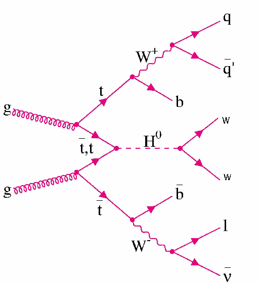
The method used to measure the Higgs CP under investigation requires full reconstruction of the event. Specifically it uses the reconstructed top momenta. This means using the reconstructed detector objects (i.e. electrons, jets etc) the 4 W's as well as the two tops and Higgs would ideally need to be fully reconstructed. Two possible final states are interesting given this requirement.
- States with more than two leptons have a branching fraction of only \( \approx \) 0.1x0.1x0.67x0.67=0.004489 and their nature make reconstruction very difficult/ impossible because of the multiple sources of missing energy from the different neutrinos in the final state.
- The two lepton final state has only two hadronically decaying W's in the final state. However, at the time this work was carried out even though methods existed to reconstruct events with more than one source of missing energy these methods were widely untested.
- The final state with no leptons doesn't allow for easy triggering and is too combinatorically challenging.
- The one lepton final state is considered here. It has the advantage of having only one source of missing energy making attributing missing energy to detector objects more error free. However, it does have three hadronically W's, each of which needs to be reconstructed and attributed to the tops and Higgs and therefore presents quite a combinatoric challenge. This aspect should however provide a means by which to discriminate backgrounds. The one lepton final state has a branching ratio of \( \approx \) 0.67x0.67x0.67x0.1=0.03.
ATLFAST fast simulation for ATLAS
ATLFAST is a software package that provides the ATLAS collaboration a means by which to quickly simulate the detector response at the particle level, through the use of a parametized detector response. It is primarily used when analysis of large datasets is required or for feasibilty studies such as this.
The first step in ATLFAST is the deposition of electron, photon and hadron energies in the calorimeter cell map. The response of the calorimeter is assumed to be 1 and uniform with no smearing applied. The granularity of calorimeter cells is set as Eqn. \eqref{eqn_granularity_2} $$ \begin{equation} \Delta \eta \times \Delta \phi = 0.1 \times 0.1 \mathrm{ for } |\eta| < 3.2 \\ \Delta \eta \times \Delta \phi = 0.2 \times 0.2 \mathrm{ for } |\eta| < 5.0 \label{eqn_granularity_2} \end{equation} $$
The electromagnetic and hadronic calorimeters are not separate. No hits or tracks are simulated in the inner detectors or muon chambers. Interations of particles with the detector medium are approximated using resolution functions.
Reconstruction of physics objects is largely reliant on Monte Carlo truth. In particular there is no reconstruction layer based on the simulated detector, apart from a seeded cone algorithm for cluster reconstruction in the calorimeter. Instead, the process of identifying physics objects is reliant on the nature of the truth particles. The process starts with the energy deposits in the calorimeters. A cluster reconstruction algorithm is used (cone algorithm with \( \Delta \) R = 0.4) to identify clusters passing a 5 \( \GeV \) threshold. Each cluster identified can then be reclassified as one of the following depending on if certain criteria are satisfied.
Electrons
For each truth electron a calorimeter cluster matching it in \( \eta \phi \) space is searched with an acceptance of \( \Delta \) R = 0.15. A cluster satisfying this criteria is defined as an isolated electron if the difference in the energy of a cone of \( \Delta \) R = 0.2 around the electron direction and smeared electron energy is below the 10 \( \GeV \) threshold. In addition, no clusters around a \( \Delta \) R = 0.4 cone of the electron direction should be present. The reconstructed electron energy is obtained by smearing the truth electrons energy with a resolution function. If this is larger than the threshold energy of the cluster and a true electron is within \( \Delta \) R < 2.5 an isolated electron is recorded. It's \( \eta \) and \( \phi \) are designated to be the same as for the truth electron to which it was matched.Muons
For each truth muon with \( \pt \) > 0.5 \( \Gc \) the reconstructed momentum is found by applying a gaussian resolution function (depending on \( \pt \) , \( \eta \) and \( \phi \) ) to the truth momentum. After this process, reconstructed muons with \( \pt \) > 5 \( \Gc \) and \( |\eta| \) < 2.5 are kept. By passing similar criteria as for electrons, a muon may then be considered as isolated or non- isolated. Muons within a \( \Delta \) R = 0.4 cone of a reconstructed jet are added to the jet.Jets
Clusters not associated to a true electron or photon are considered as jets if the transverse energy exceeds a threshold of 10 \( \GeV \). The jet energy from the cluster energy is smeared using a resolution function as shown in Eqn. \eqref{eqn_granularity_3}. $$ \begin{equation} \frac{\sigma}{E} = \frac{50\%}{\sqrt{E}} \oplus 3\% \mathrm{ for } |\eta| \leq 3.2 \frac{\sigma}{E} = \frac{100\%}{\sqrt{E}} \oplus 7\% \mathrm{ for } 3.2 < |\eta| < 4.9 \label{eqn_granularity_3} \end{equation} $$The direction of a jet is assumed to be the direction of the cluster. A jet is called a bjet if at event generator level (after FSR) a b quark lies within \( \Delta \) R < 0.2 and has \( \pt \) > 5 \( \Gc \). A similar procedure is used for c jets.
Missing momentum
Missing transverse momentum is calculated using reconstructed objects and calorimeter cells not associated to clusters whose energies are smeared with a jet resolution function.Event Pre - Selection
In this section we present the event reconstruction cuts put in place due to detector requirements, to maximise signal to noise ratio and those imposed due to the proposed method to measure the Higgs CP parity. These steps are performed before the reconstruction the event.
- Cut0: Standard cuts on pseudo-rapidity (\( \eta \)) of jets and leptons, taking into account limits in detector spatial coverage are implemented, requiring (light) jets have \( |\eta| \) < 2.5, while b-tagged jets and leptons are restricted to \( |\eta| \) < 2.5.
- Cut1: Select events with only one lepton.
- Cut2: The next cut is on number of b tagged jets. Two methods have been developed to deal with events of two classes.
- Events with two or more b tagged jets. The two highest \( \pt \) b tagged jets are used for the expected b tagged jets in the event and the other ones considered when recontructing the decaying hadronic W's.
- Events with one b tagged jet (i.e. one mis-identified). In this case the mis-identified b tagged jet is considered to be the highest \( \pt \) non b-tagged jet.
- Cut3: Allowing for three hadronic W's decaying to two light jets each and two(one) b tagged jets, each event must have at least 6(7) light jets (each with \( \pt \) > 15 \( \Gc \)) to be reconstructed.
Reconstruction of the \( \tthtoWW \) topology
Reconstruction of the leptonically decaying W
The following is done after the lepton selection, before the selection of jets is made. In order to be able to fully reconstruct the event, the neutrino (resulting from the leptonically decaying W) momentum must be retrieved even though this is not measureable directly in the detector because neutrinos interact very weakly. However, because the initial state of two hard scattering partons has zero transverse momentum, the neutrino transverse momentum can be measured indirectly through the imbalance of \( \pt \) in the final state, i.e. measured missing transverse momentum. However \( p_{z\nu} \) is not known since the \( p_{z} \) of the initial partons is unknown. This can however be resolved with the following ideas:- The sum of the lepton and neutrino momentum is equal to the W momentum.
- If the mass of the neutrino-lepton system is constrained to the measured W mass, then a quadratic equation for \( p_{z\nu} \) results as shown in Eqn. \eqref{te}.
- Method 1: Set the term inside \( \sqrt{} \) to 0 and calculate \( p_{z\nu} \) accordingly.
- Method 2: Set \( p_{z\nu} \) to \( p_{z lepton} \) (collinear approxmiation).
Figure 2: a) \( \Delta \) R between truth and reconstructed leptonic W and b) mass of reconsructed lepton+neutrino system.
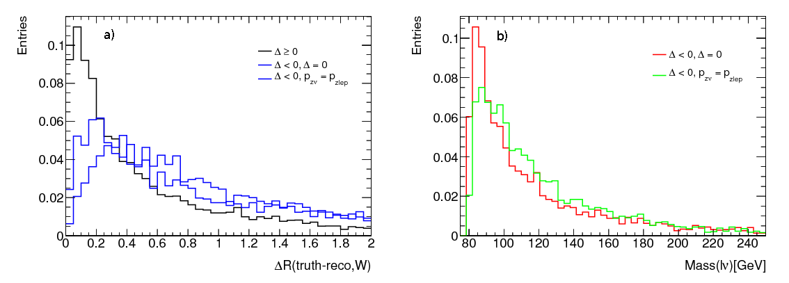
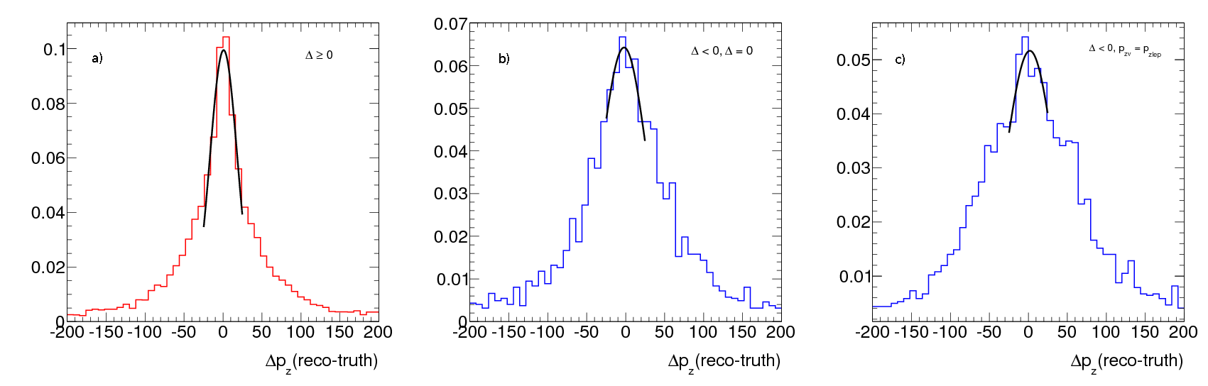
Figure 3: Comparison of performance of \( p_{z\nu} \) resolution for events with (a) real solution of quadratic quation, no real solution to quadratic quation using approximation (b) \( \Delta \) = 0 and (c) \( p_{z\nu} \) = \( p_{z lepton} \) .
Reconstruction of the hadronically decaying W's
The events considered, determined from the need to accurately reconstruct top momenta, have large light jet multiplicities, with an average of about ten light jets for events with two b tagged jets as shown in Figure 4.
Figure 4: Jet multiplicities for \( \tthtoWW \) events with 1 leptonically decaying W
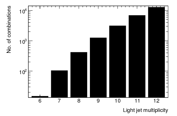
Due to limited statistics and desire to test (optimize) the effect of consideration of different numbers of light jets, the event reconstruction technique needed be able to deal with all numbers of light jets, from the threshold required by the event pre-selection to the total number of light jets in the event. Essentially this means the method must be able to deal with the large combinatorics that come from consideration of all possible unique pairings of \( n \) light jets to three hadronic W's. Depending on \( n \), the number of ways of pairing the light jets to the three hadronic W's is shown in Eqn. \eqref{eqn_ncomb} $$ \begin{equation} \ncomb = \frac{1}{6}\frac{n_{ljets}x(n_{ljets}-1)}{2}\frac{(n_{ljets}-2)x(n_{ljets}-3)}{2}\frac{(n_{ljets}-4)x(n_{ljets}-5)}{2} \label{eqn_ncomb} \end{equation} $$
(where \( \nolj \) = number of light jets per event). Two tests were performed to verify that the code is considering all correct combinations. First the total number of combinations found by the code produced was compared to that computed using Eqn. \eqref{eqn_ncomb}. Agreement was found when between 6 and 20 light jets were considered. Second, for a number of different scenarios (6,7,8 light jets), the combinations considered by the code were compared to those computed manually. Agreement was found in all cases.
Reconstruction Methods
The reconstruction of the event was performed in two steps:- First the different combinations are built including association of light jets to W's to build up the three hadronic W's.
- Next the process of reconstructing the tops and Higgs is done by associating a W to a b tagged jet for each top and two W's for the Higgs.
Reconstruction using a \( \chisq \)
This method compares each possible association using a \( \chisq \), using the known masses of the top quarks and W bosons to constrain the combinations. A five component \( \chisq \) as shown in Eqn. \eqref{eqn_chi2_1} was initially used, where three terms account for the hadronic W's and two terms are used for the two top quarks. $$ \begin{equation} \chisquared \label{eqn_chi2_1} \end{equation} $$ where \( i,j,k,l,m \) and \( p \) are light jet pairs from the three hadronic W's (i.e. each \( ij \) , \( kl \) , \( mp \) is one contribution to Eqn. \eqref{eqn_ncomb} ), \( \sigma_{W} \) and \( \sigma_{t} \) are the W and top mass resolutions, \( m_{W} \) and \( m_{t} \) are the input W and top masses and \( index1 \) and \( index2 \) are indices over all unique pairings of four reconstructed W's to two b jets to make two top quarks. All combinations are evaluated and the one giving the minimum value is chosen.
To further contrain the combinations a Higgs boson term was added resulting in a six component function of the form shown in Eqn. \eqref{eqn_chi2_2}. $$ \begin{equation} \chisquaredwithhiggs \label{eqn_chi2_2} \end{equation} $$
where index3 refers to the W's not used by the tops (i.e. given a specific \( index1 \) and \( index2 \)), \( m_{h} \) = 160 \( \Gcs \) and \( \sigma_{h} \) was set equal to \( \sigma_{t} \). The purpose of this implementation was to test whether the method is feasible at reconstructing the event (it essentially gives the best result that is possible by including all information).
For each distinct pairing of light jets to hadronic W's (i.e. a given \( ij \) , \( kl \) , \( mp \) set) and leptonic W solutions, there exist a number of ways in which the W's and b jets can be paired to make tops and Higgs candidates. Because every event considered has one leptonic W and three hadronic W's, the events can be divided into two classes, those with a semi-leptonic top or those where one of the Higgs W's decays leptonically.
For example, for events with a semi-leptonic top, 12 different \( \chisq \) must be considered (two b tagged jet events). For events where one of the Higgs W's decays leptonically, a further six different \( \chisq \) must be considered (if Higgs term in the \( \chisq \) is excluded. For such events, the leptonic W solution is not constrained and the one giving a resulting Higgs mass closer to the generated mass of 160 \( \Gcs \) is chosen).
The resulting signal and combinatoric background output for combinations with the quantities with the two tops matching using the \( \chisq \) method with the Higgs term is shown in figure 5.
Figure 5: Reconstructed top and Higgs masses (including signal and combinatoric background as identified by the \( \chisq \) method) for semi-leptonic top events (top row) and semi-leptonic Higgs events (bottom row).
Multivariate reconstruction method- boosted decision tree
The boosted decision tree takes into account correlations between variables, useful in a complicated topology like the one considered. A boosted decision tree (BDT) is a machine learning algorithm based on recursive growth of a tree like diagram where at each node a decision is made. The node is defined as a signal leaf node or a background leaf node or additional cuts are required to allow a discrimination to be made. When training, signal and background are treated as totally separate and as such correlations in the same event are not taken into acocunt, i.e. for a given combination, the classifier is not aware of the properties of the other combinations. For the BDT the correct combination corresponds to a recontructed combination chosen using truth \( \Delta \) R matching. The variables used for the multiariate input discriminating variables are:Semi-leptonic top events:
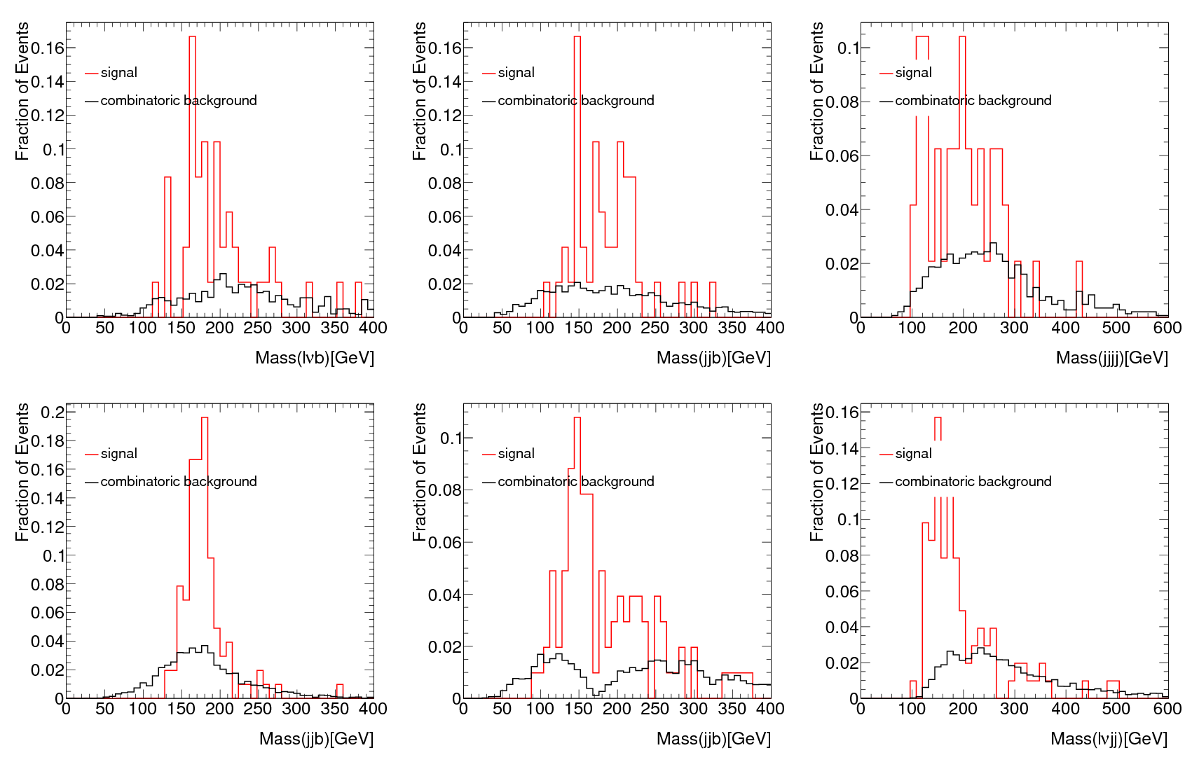
- Mass(jj): Invariant mass of the hadronic W decay from the top.
- \( \Delta \) R(jj): angle between the jets used to recontruct the hadronic W from the top.
- Mass(jjb): Invariant mass of the hadronic top decay products.
- \( \Delta \) R(jjb): \( \Delta \) R between the reconstructed hadronic W and the b-jets associated with the hadronic top.
- Mass(l \( \nu \) b): Invariant mass of the leptonic top decay products.
- \( \Delta \) R(l \( \nu \) b): \( \Delta \) R between the reconstructed leptonic W and the b-jets associated with the leptonic top.
- Mass(l \( \nu \) b \( _{\mathrm{hadronic}} \) ): Invariant mass of leptonic W and b-jets associated with the hadronic top.
- \( \Delta \) R(l \( \nu \) b \( _{\mathrm{hadronic}} \) ): \( \Delta \) R between the lepton and the bjets from the hadronic top.
- Mass(jjb \( _{\mathrm{leptonic}} \) ): Invariant mass of hadronic W and b-jets associated with the leptonic top.
- \( \Delta \) R(jjb \( _{\mathrm{leptonic}} \) ): \( \Delta \) R between the hadronic W and the bjets from the leptonic top.
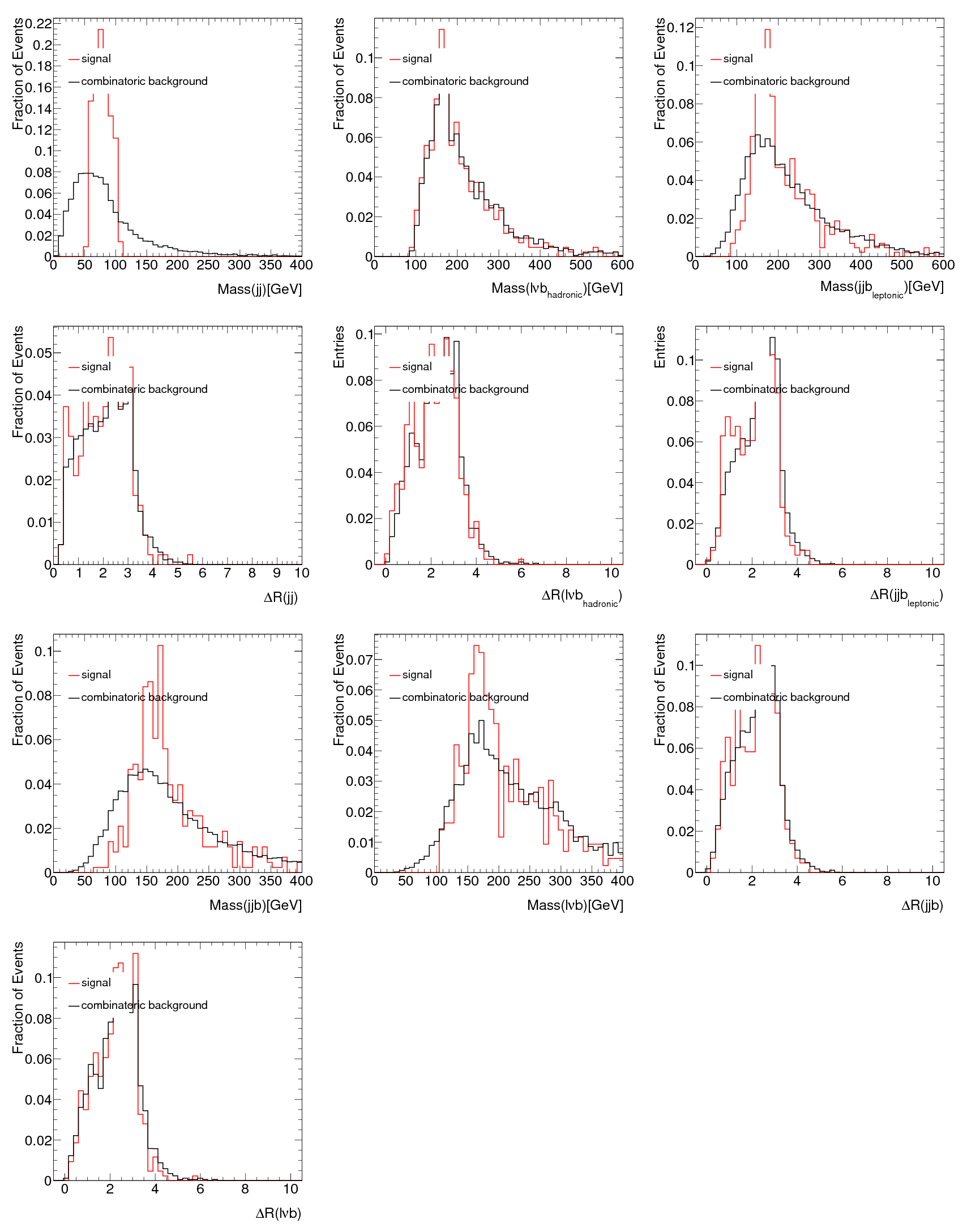
- Mass(jj): Invariant mass of the hadronic W decay from the top.
- \( \Delta \) R(jj): angle between the jets used to recontruct the hadronic W from the top.
- Mass(jjb): Invariant mass of the hadronic top decay products.
- \( \Delta \) R(jjb): \( \Delta \) R between the reconstructed hadronic W and the b-jets associated with the hadronic top.
- Mass(l \( \nu \) b): Invariant mass of the leptonic top decay products.
- \( \Delta \) R(l \( \nu \) b): \( \Delta \) R between the reconstructed leptonic W and the b-jets associated with the leptonic top.
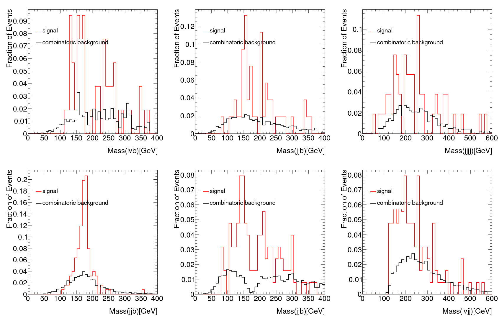
Figure 6: Discriminating variables used as input for BDT for semi-leptonic top events, showing identified signal and combinatoric background.
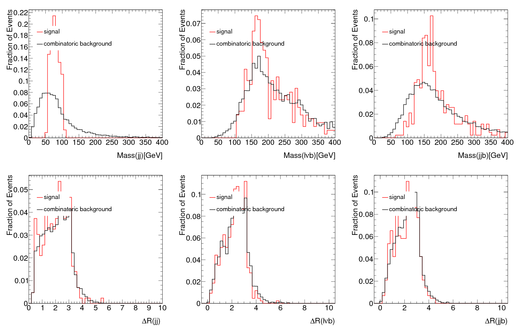
Figure 7: Discriminating variables used as input for BDT for semi-leptonic Higgs events, showing identified signal and combinatoric background.
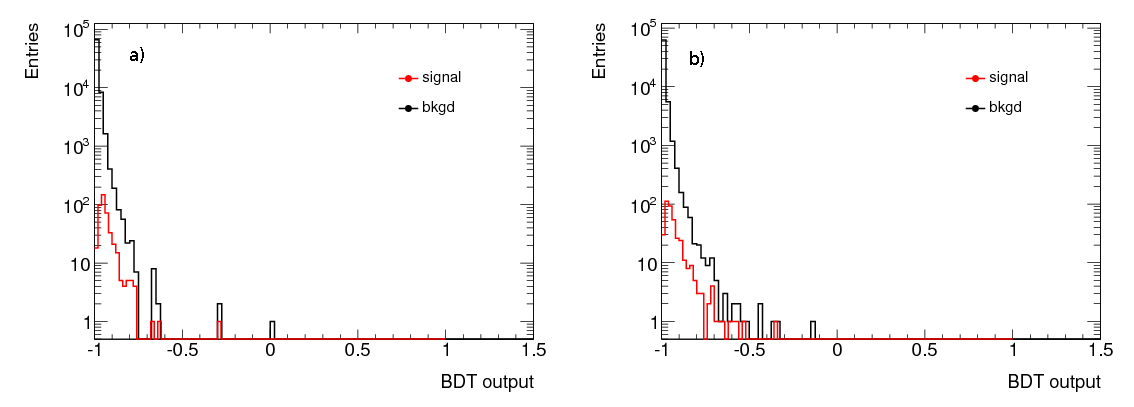
The TMVA implementation of the BDT is used [4]. Most variables are default athough a few are altered to avoid overtraining. The output of the BDT for signal and background is shown for semi-leptonic top events in Figure 8a) and for semi-leptonic Higgs events in Figure 8b)
Figure 8: BDT output for signal and combinatoric background a) for semi-leptonic top events and b) semi-leptonic Higgs events.
The reconstructed masses for the tops and Higgs for semi-leptonic top and semi-leptonic Higgs events (including identified signal and combinatoric background) are shown in Figure 9.
Figure 9: Reconstructed top and Higgs masses (including signal and combinatoric background as identified by the BDT method) for semi-leptonic top events (top row) and semi-leptonic Higgs events (bottom row).
Results and conclusions
A comparison of the methods and different classes of events is shown in the table below. It shows the percentage of events from the test set, of the class indicated, where the signal combination chosen by either method, matches the combination chosen by truth matching.
| Quantity | Method | ||
| \( \chisq \) with higgs | BDT | ||
| semi leptonic top | hadronic top | 19.6 \( \mypm \) 3.7 | 34.5 \( \mypm \) 5.3 |
| events | leptonic top | 27.5 \( \mypm \) 4.6 | 25.2 \( \mypm \) 4.3 |
| Higgs | 11.9 \( \mypm \) 2.8 | 22.1 \( \mypm \) 4.0 | |
| both tops | 11.2 \( \mypm \) 2.7 | 12.4 \( \mypm \) 2.9 | |
| 2 tops and Higgs | 7.0 \( \mypm \) 2.1 | 8.9 \( \mypm \) 2.4 | |
| semi leptonic Higgs | hadronic top 1 | 38.3 \( \mypm \) 6.8 | 44.6 \( \mypm \) 7.6 |
| events | hadronic top 2 | 41.3 \( \mypm \) 7.2 | 45.4 \( \mypm \) 7.6 |
| Higgs | 20.2 \( \mypm \) 4.6 | 22.4 \( \mypm \) 4.9 | |
| both tops | 26.0 \( \mypm \) 5.4 | 32.1 \( \mypm \) 6.1 | |
| 2 tops and Higgs | 14.5 \( \mypm \) 3.7 | 14.5 \( \mypm \) 3.8 |
Clearly the results are statistically limited. However, they do indicate that the BDT approach used yields an improvement in the reconstruction efficiency, particularly for certain classes of event.
Bibliography
- S. McGarvie. \( \toptop \) (H \( \rightarrow \) 2 \( \gamma \) ) Search and CP Measurement, (unpublished), 2006.
- N. Andari et al.. Higgs Production Cross Sections and Decay Branching Ratios, ATLPHYSINT2011049, 2010.
- S. L. Glashow. Partial Symmetries of Weak Interactions, Comput. Phys., 22, pp. 579-588, doi: 10.1016/0029-5582(61)90469-2, 1961.
- A. Hoecker. TMVA, Toolkit for Multivariate Data Analysis, ArXiv Physics e-prints, 2007.