Searching for the Higgs Boson with the ATLAS detector at CERN

Clive Edwards (mail at cedwards.info)

Summary. This report summarises the particle physics project the author performed which aimed at searching for evidence of the Higgs boson using large quantities of Monte Carlo simulated data and real data from the ATLAS experiment at CERN.

The search potential of a Standard Model Higgs boson in the Vector Boson Fusion production mechanism with Higgs boson decaying to two leptons and two neutrinos via decay to two Z bosons with the ATLAS detector is investigated. The ATLAS detector is a general purpose detector in operation at CERN measuring proton-proton collisions produced by the Large Hadron Collider. This channel has been shown to have high sensitivity at large Higgs mass, where large amounts of missing energy in the signal provide good discrimination over expected backgrounds. This work takes a first look at whether the sensitivity of this channel may be improved using the remnants of the vector boson fusion process to provide extra discrimination, particularly at lower mass where sensitivity of the main analysis is reduced because of lower missing energy.

Simulated data samples at centre of mass energy 7 TeV are used to derive signal significances over the mass range between 200-600 $ \Gcs $. Because of varying signal properties with mass, a low and a high mass event selection were developed and optimized. A comparison between simulated and real data (collected in 2010) is made of variables used in the analysis and the effect of pileup levels corresponding to those in the 2010 data is investigated. Possible methods to estimate some of the main backgrounds to this search are described and discussed. The impact of important theoretical and detector related systematics are taken into account. Final results are presented in the form of 95 $ \% $ Confidence Level exclusion limits on the signal cross section relative to the SM prediction as a function of Higgs boson mass, based on an integrated luminosity of 33.4 $ \pb $ of data collected during 2010.

Skills used:

Data cleaning (see the section Physics Objects) (cross checking of simulated (Monte Carlo) and real data, and where neccessary making modifications to Monte Carlo (i.e. accounting for detector effects and pile-up)).
Feature Selection (See the sections Feature Selection Signal and Background Processes) (development of two cut based selections as a function of Higgs mass in order to extract Higgs signal and from its backgrounds- based on physics and cross checking distributions).
Big Data Analysis (see the section Signal and Background Processes for description of some data samples used) (analysis of multiple $ \approx $ TB's size datasets using the CERN world wide computing Grid, batch analysis with qsub).
Optimization (see the section Optimization of Feature Selection cuts) (of feature selection yielding approximately 10 $ \% $ improvement in signal sensitivity relative to baseline selection.
Algorithm development (Individually wrote all code used in the analysis phases of the study, including multidimensional optimization code).
Statistics (see the section Results in form of Limits) (hypothesis testing).
Data Visualisation and documentation (workflow, analysis and presentation of results- CERN ROOT, $ \LaTeX $ ).
Linux (study was entirely performed on linux computers, most of the time accessed remotely through terminal).
End to end analysis (in depth study with real aims and outcomes).
Data migration (analysis was done using various formats at different stages- Monte Carlo and data from data sets containing all information from detector was reduced in size by recording desired information- allowing for more efficient analysis).
Programming (C++, Python, make).
Mathematics.
Version control (SVN).

Motivation

The Higgs boson was predicted theoretically to exist by Peter Higgs [1] and others [2] [3] in 1964. It forms an intricate part of our framework for understanding elementary particles and their interactions. Arguably it was the main motivation that prompted the construction of the LHC and associated experiments, CMS and ATLAS, who purpose it would be to find experimental evidence for the existence of such a particle. The CMS and ATLAS detectors are in essense gigantic microscopes which allow, through colliding very high speed (energy) protons (provided by the LHC) together in their centre, researchers to investigate the fundamental consistuents of matter and the forces between them. The energies at which the protons collide at the LHC were and remain at the highest energies anywhere in the world, allowing access to the 'small scale' at which evidence for the Higgs boson could be found experimentally. In essence, when large numbers of high energy protons are collided together, because in part of their non-fundamental nature (they themselves are made of constitent parts), the end product is a very messy mix of particles, with a huge number of different possible outcomes depending on the physics properties of the individual collisions. Producing a Higgs boson has a very small chance of happening theoretically, compared to the mutlitude of other more probable processes. The mathematics behind the theory of the Higgs boson and of elementary particle theory predicts the Higgs boson can only be detected by its decay products or what it 'turns into'. Indeed there are numerous theoretically predicted so called decay channels for the Higgs boson. In addition there are a number of methods by which it can be produced. Therefore using the ATLAS detector at CERN to search for the Higgs boson is very much like the analogy of 'searching for a needle in a haystack'. In essence the problem can be defined as using vast amounts of data to find statistical evidence for a signal (the Higgs boson) amoungst the much more numerous background of particles produced by the much more numerous other processes occuring at a much higher rate.

As is still currently the case, our theoretical understanding of all these processes is modelled using the Monte Carlo simulation, which not only simulates each physical process resulting from the proton-proton collisions, right the way to the final particles 'seen' in the detector, it also has the ability to take into account the modelling of these particles as they travel through the detector. By comparing this theoretical representation (in all the different production and decay modes) to actual data recorded by the detector and stored for later use, theoretical ideas can be tested, as was subseqeuntly done in 2012 when the Higgs boson was discovered to the 5 $ \sigma $ level (i.e. an excess of events with a statistical significance of five standard deviations above background expectations). The search the author was involved in occured prior to this, when much less data had been taken by the experiments, yet non the less important work could be done. The search focussed on a particular form of Higgs boson, predicted to be produced in a certain way (vector boson fusion), and subseqent decay (to two Z bosons), giving rise to a so called final state, detectable in the detector, of two jets, two leptons and two neutrinos. It was the first search performed within the ATLAS experiment of its kind.

Introduction

The Standard Model of Particle Physics

Elementary particles and their interactions

Our current understanding of the physical world in terms of fundamental matter particles and their interactions is largely based on the Standard Model (SM) of particle physics. It describes all known particles and three of the four known fundamental interactions (the electromagnetic, weak and strong interactions). Within the SM the particles are classified by their spin as either

half-integer spin particles called fermions obeying Fermi-Dirac statistics. These form the matter particles.
integer spin particles called bosons. These particles obey Bose-Einstein statistics and their exchange between the fermions describes the fundamental interactions.

The fermions are categorised into two types, the quarks and the leptons. The quarks are given a baryon number B=1/3. The leptons are assigned a lepton number L=1 and do not interact via the strong interaction. Each type of fermion consists of three families or generations, each of which consists of two distinct particles (often referred to as a doublet of particles). Figure 1 lists the quarks and leptons and some of their basic properties [4].

Figure 1: The fermions and some of their basic properties. Masses are given in $ \Gcs $ (the electron volt is a unit of energy, so this unit for mass comes from rearranging E=m c $ ^{2} $ ) and the electric charge in units of the electrons charge, $ |e| $ [4]

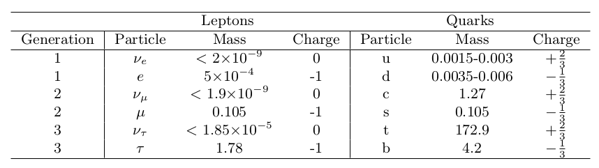
The first generation of quarks consists of the up (u) quark with + $ \frac{2}{3} $ electric charge (in units of electron charge, $ |e| $) and the down (d) quark with -$ \frac{1}{3} $ electric charge. The other generations consist of a u-type and a d-type quark but are successively heavier than the first generation. The second generation consists of the strange (s) and charm (c) quarks while the third generation consists of the bottom (b) and top (t) quarks. Quarks carry colour charge and as such each comes in three distinct colour states (red, green or blue). Each doublet of leptons is composed of an electrically charged lepton and its corresponding neutral neutrino. As with quarks, the mass of the charged leptons in the doublet increases with generation. The first generation consists of the electron ($ e $) and its neutrino ($ \nu_{e} $), the second the muon ($ \mathrm{\mu} $) and its neutrino ($ \nu_{\mu} $) and the third the tau ($ \mathrm{\tau} $) and its neutrino ($ \nu_{\tau} $). Each quark and lepton have a corresponding anti-particle, denoted with a bar. Anti-particles have opposite electric charge to the corresponding particle but the same mass. In nature quarks are only found within composite hadrons, composed of either three quarks making a baryon or in quark anti-quark states called mesons.

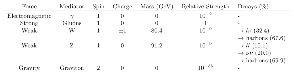
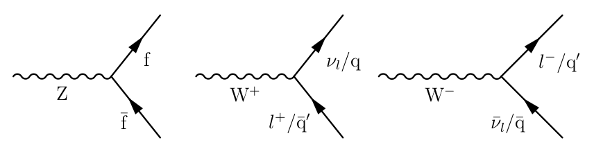
Interactions between the fermions are mediated by the absorption and emission of integer spin particles called bosons. This gives rise to four fundamental forces, summarised in Figure 2. The electromagnetic force makes the electron bind to nuclei and more generally, molecule formation underpinning Chemistry. It is mediated by the photon ( $ \gamma $ ). The strong force is responsible for holding nuclei together and is mediated by eight massless gluons (g). The weak force explains $ \beta $ decay and is mediated by exchange of W $ ^{+/-} $ and Z bosons. Gravity is responsible for galactic formation. It is the weakest of all the forces and is negligible at the energy scales considered in particle physics. In principle, gravity can be described as being mediated by the exchange of a boson called the Graviton.

Figure 2: The mediators of the four fundamental fermion interactions and some of their basic properties. Relative strength corresponds to the typical strength of the forces compared to the strong force between two protons separated by $ \approx $ 15 $ \mathrm{fm} $ [5]. Here $ l $ refers to lepton ( $ e,\mu,\tau $ ).

The Standard Model

The SM is a theoretical framework of quantum field theory [6] in which the elementary particles are the quanta of the underlying fields and the interactions are a consequence of the principle of local gauge invariance. As yet attempts to incorporate gravity using this approach have failed. The time-line of the SM becoming a unified theory of the forces that it describes started with the development of the quantum field theory of electromagnetic interactions, called Quantum Electrodynamics. Subsequently in the 1960's a unified electroweak theory was developed unifying the electromagnetic and weak interactions. Finally the electroweak theory was unified with the theory of the strong interactions (Quantum Chromodynamics) giving what is understood as the SM today. Doing this in the conventional way led to the requirement that the bosons be massless, something which we know not to be the case from experimental observations.

Quantum Electrodynamics

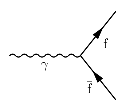
All quantum electromagnetic interactions consist of the interaction of charged fermions with the quantum of the electromagnetic field, the photon, and are encompassed within Quantum Electrodynamics (QED). The most basic form of such an interaction, is shown in Figure 3. It shows the interaction of a charged fermion f with a photon $ \gamma $. As with all interactions, the strength is characterized by a coupling constant associated to each vertex. The electromagnetic force couples to electric charge and so this defines the strength of electromagnetic interactions. This vertex corresponds to the basic building block from which all QED processes can be represented. Complete QED processes represented in this way are called Feynman diagrams. Feynman diagrams with the smallest number of vertices for a given process to occur are referred to as tree-level or leading-order whereas diagrams with a higher number of vertices are called higher order diagrams. Feynman diagrams without internal loops are referred to as tree-level or leading-order whereas diagrams with internal loops are called higher order diagrams. A detailed picture of any QED process can be obtained by summing over all possible internal states and this corresponds to summing over all Feynman diagrams of all orders.

Figure 3: The basic QED vertex involving a $ \gamma $ and a charged fermion f.

Quantum Chromodynamics

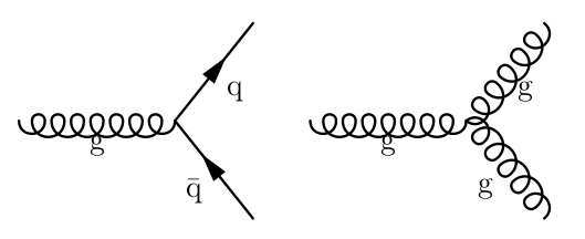
Quantum Chromodynamics (QCD) is the quantum field theory describing the strong interactions. The strong force couples to colour charge, so only the coloured gluons and quarks are involved in strong interactions. The most basic QCD interaction vertex, involving the interaction of quarks (q) with a gluon (g) is shown in leftmost figure in Figure 4.

Figure 4: Basic QCD interaction vertices involving (left) gluon (g) and quark (q) anti-quark ($ \antiquark $) and (right) gluon self interaction.

Weak and Electroweak Interactions

The basic allowed weak interaction vertices are shown in Figure 5.

Figure 5: Weak interaction vertices allowed in the SM.

The Higgs Mechanism

The mechanism of spontaneous electroweak symmetry breaking applied to a $ non-abelian $ theory was introduced by Peter Higgs [1] and others [2] [3] in 1964 and provides a solution to the massless fields (bosons). This is what is commonly known as the Higgs mechanism. The Higgs boson mass is a free parameter in the SM and as such cannot be predicted. Despite this there exist a number of ways to constrain its mass broadly speaking coming from theoretical and experimental means. The experimental constraints on the Higgs bosons mass come from searching for its production, by colliding particles at high energy in particle colliders.

The LHC began operation in 2009 operating at $ \sqrt{s} $ = 7 $ \TeV $ and since then searches for the SM Higgs boson utilizing data have become established. As of summer 2011 the ATLAS Collaboration, using a combination of search channels each using between 1.0 to 2.3 $ \fb $ of data, produced preliminary results [7] indicating exclusion of the Higgs boson mass ranges from 146 $ \Gcs $ to 232 $ \Gcs $, 256 to 282 $ \Gcs $ and 296 to 466 $ \Gcs $ at the 95 $ \% $ C.L.. In the absence of a signal the expected Higgs boson mass exclusion ranges from 131 to 447 $ \Gcs $. The CMS Collaboration also presented similar results in summer 2011.

Higgs production at the LHC can be divided into four main mechanisms, gluon gluon fusion (GF) ( $ \glgl \rightarrow $ H), Vector Boson Fusion (VBF) ( $ \qq \rightarrow \qq $ H), associated production with W/Z boson ( $ \qq \rightarrow $ HW/Z) and associated production with heavy quarks ( $ \glgl/\qq \rightarrow \qq $ H). Feynman diagrams showing each of these processes are shown in Figure 6.

Figure 6: Diagrams of SM Higgs Production Modes at the LHC.

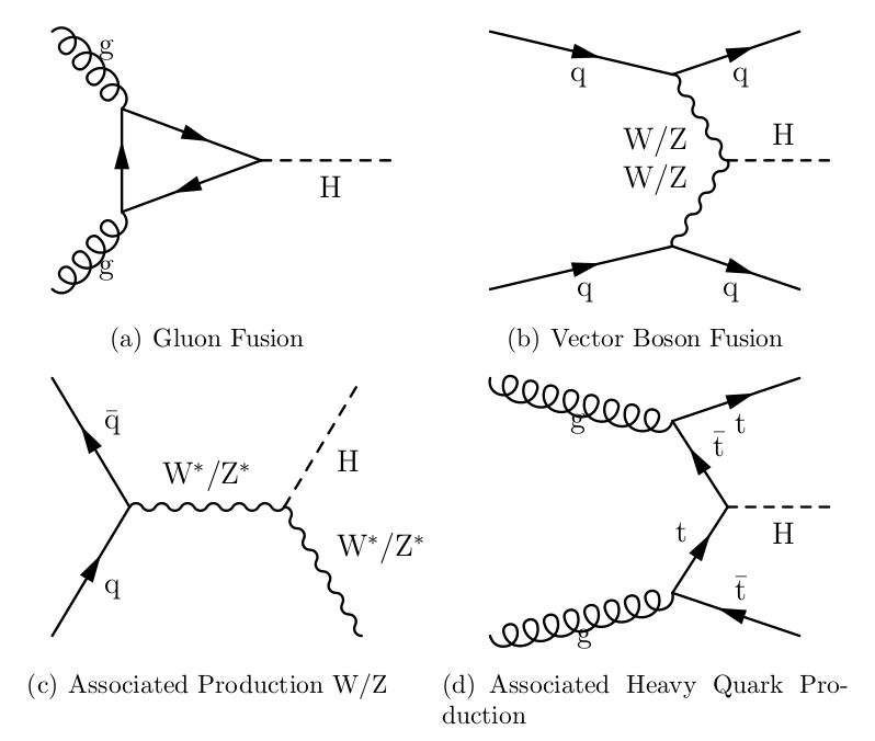
GF mediated by heavy quark loops is the dominate production mode. This is largely due to higher order QCD corrections, with next-to-leading order (NLO) effects increasing its total cross section by $ \sim $ 80-100 $ \% $ at the LHC [8].

VBF is suppressed by approximately one order of magnitude compared to GF according to the SM. However this mode of production produces a Higgs boson in association with two quarks, leading to the production of two highly energetic jets typically in the forward regions of the detector with no jet activity other than that produced from the Higgs decay products between them (because of no colour flow between the initial interacting particles). This results in a distinctive signal signature allowing for efficient suppression of backgrounds. The associated production modes have lower cross section than either GF or VBF. Nonetheless they will need to be studied in order to verify the validity of the SM prediction of Higgs production modes. In addition associated production with heavy quarks is important for measuring the properties of the Higgs boson.

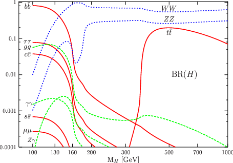
The decay of the Higgs boson according to the SM can be loosely grouped into decays to fermion and gauge boson pairs (and virtual loops). The branching ratios (BR) or relative rates of the SM Higgs boson for each decay mode, as a function of Higgs mass, are shown in Figure 7. At tree level, the coupling strength of the Higgs boson to fermions is proportional to the mass of the particles concerned. The net result is that a Higgs boson of a given mass will decay to the heaviest fermions that are kinematically accessible and as a consequence the decays of the Higgs boson can be further classified by Higgs mass.

Figure 7: Branching ratios for the SM Higgs boson as a function of its mass [9].

The Large Hadron Collider

The Large Hadron Collider (LHC) is a proton-proton (pp) collider with design centre of mass energy $ \sqrt{s} $ = 14 $ \TeV $ and is the successor of the LEP collider. It has a 26.7 km circumference and is constructed approximately 100 m below ground level, on the Swiss-French border, installed in the existing tunnel used by the LEP collider. Its design characteristics are shown in Figure 8.

Figure 8: Main LHC parameters.

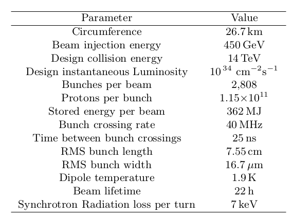
Being a pp collider, the LHC's maximum $ \sqrt{s} $ (like the Tevatron's) is not limited by synchrotron radiation (power emitted proportional to $ 1/m^{4} $ where $ m $ = beam particle mass) as was the case for the LEP collider. However, the production of antiprotons is highly inefficient so the LHC accelerates two counter rotating proton beams. This feature means that in contrast to $ \ppbar $ colliders such as the Tevatron where both beams can share the same beam pipe, the LHC needs individual beam pipes for each beam, with opposite bending magnetic field orientations. Constraints as to the size of the accelerator, imposed by the diameter of LEP tunnel, meant that a twin-bore dipole magnet design, first proposed by J. Blewett [10], was adopted.

Altogether there are six experiments at the LHC, four of which ATLAS (A Toroidal LHC ApparatuS) [11], CMS (Compact Muon Solenoid), LHCb (LHC beauty) and ALICE (A Large Ion Collider Experiment) are located in dedicated caverns underground one at each of the four interaction points of the LHC. The two other experiments, LHCf and TOTEM are situated approximately 100 m from the interaction points of ATLAS and CMS respectively. ATLAS and CMS are the LHC's two multi-purpose experiments and are the central tools that will be used to fulfil the LHC's main physics objectives, including making precision measurements of the SM, finding evidence for a Higgs-like boson and exploring physics beyond the SM. However the other detectors also have important roles. LHCb will study B Physics and CP violation in the quark sector using b-hadrons. ALICE will search for evidence of quark-gluon plasma during LHC lead-ion collision runs. TOTEM will perform measurements of the pp cross section at the LHC while LHCf will study physics at small angles to the beam direction.

The rate of proton-proton interactions (called the event rate, R) caused by the collision of the counter-rotating proton beams at the LHC is proportional to the instantaneous luminosity $ \mathcal{L} $ through $ \mathrm{R} = \mathcal{L}\sigma $, where $ \sigma $ corresponds to the event cross section or the probability of a particular interaction to occur (typically measured in barns). The LHC has a design luminosity of 10 $ ^{34} \Lum $. Two luminosity phases are scheduled at the LHC, a low luminosity phase at $ \approx $ 10 $ ^{33} \Lum $ prior to a high luminosity phase when it is expected the LHC will be run at its design luminosity of 10 $ ^{34} \Lum $. Based on the machine being kept operational for 200 days per year, the low and high luminosity phases will deliver approximately 10 and 100 $ \fb $ of data for the LHC experiments respectively.

Because increasing luminosity by increasing bunch crossing frequency puts high demands on experiment sub-detector electronic readout systems and trigger systems used to identify interesting processes, the high LHC luminosity will be achieved by increasing the density of protons per bunch, leading to multiple interactions per bunch crossing (called pile-up). When operated at its design luminosity, a nominal LHC beam will consist of approximately 2800 bunches spaced 25 ns apart and each containing around 10 $ ^{11} $ protons, giving an event rate of 40 MHz at each interaction point. This will lead to on average approximately 23 inelastic pp collisions per bunch crossing (pile-up events).

The ATLAS Detector

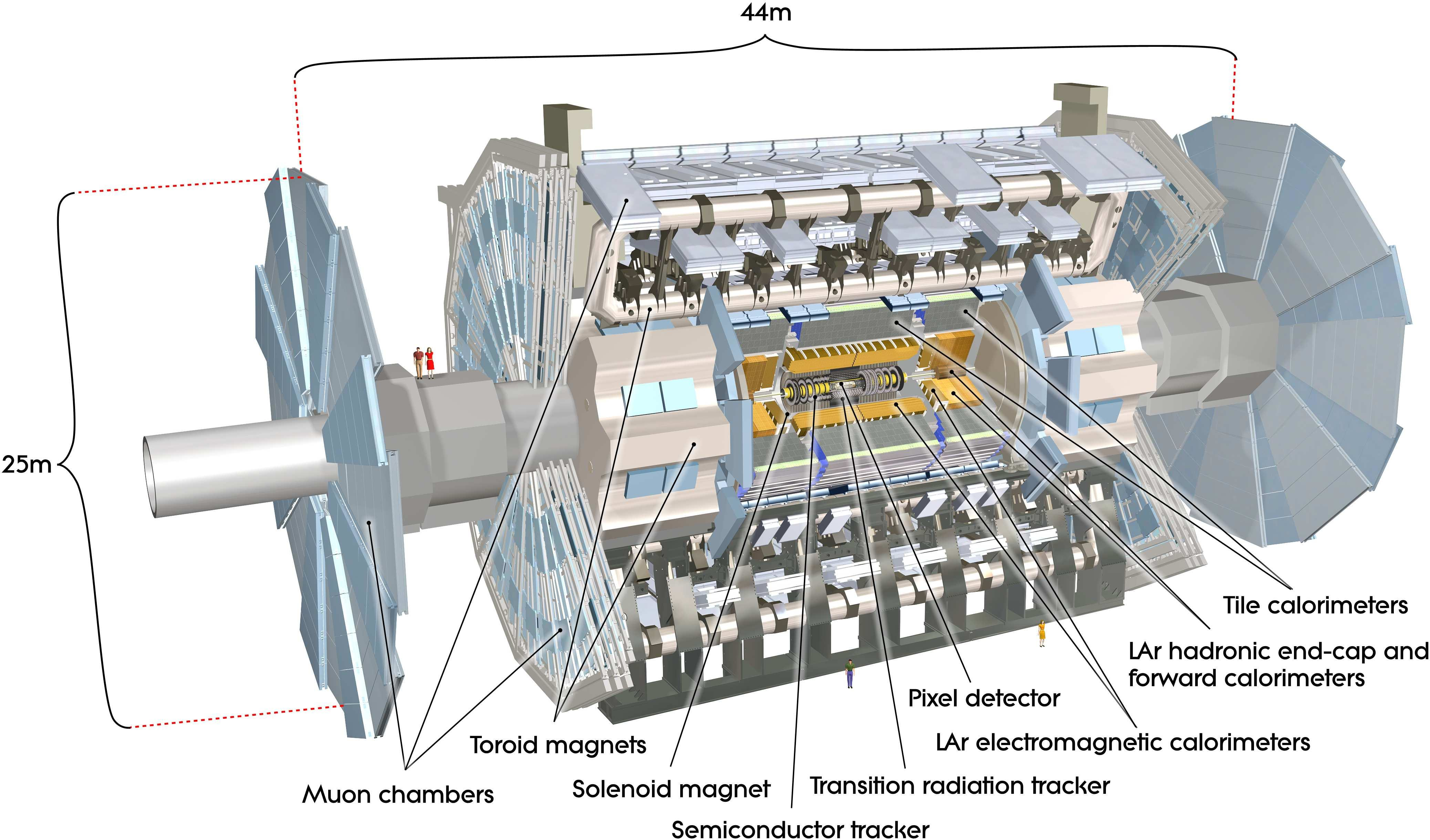
ATLAS [12] [13] is one of the two general purpose detectors at the LHC. It is designed to detect the remnants of the high energy collisions produced by the LHC in order to test our current theoretical understanding of particle interactions. In order to do this, the remnants of the collisions must first be reconstructed into meaningful particle representations, from which the different physics processes of interest can be identified. Particle reconstruction in this context is explored in more detail in the section Physics Objects.

Arguably the primary goal of ATLAS (and CMS) is to establish the cause of spontaneous symmetry breaking in the electroweak sector, and as such its design has been guided and optimized to search for a Higgs-type boson. However the unprecedented energy and luminosity of the LHC means that ATLAS's physics programme also includes

Precise SM measurements. Due to their large cross sections, W and Z bosons are produced copiously at the LHC and precision measurements of their properties have helped in the commissioning of ATLAS as well as providing a consistency check of the SM. The top quark was discovered at the Tevatron in 1995 and many of its properties studied. These will further be verified at the LHC, where the top-quark production cross section is more than two orders of magnitude higher than at the Tevatron. This is further motivated because top backgrounds will be dominant for many searches/measurements at the LHC.
Beyond the SM: Several theories predict new physics at the $ \TeV $ scale. Supersymmetry is a popular candidate. In addition, the W $ ^{'} $ and Z $ ^{'} $ bosons are examples of new particles predicted in this energy regime. Typically they decay to high $ \pt $ leptons.

A schematic layout of the ATLAS detector is shown in Figure 9, including each of its major sub-detectors. It shows ATLAS as having a layered composition with each detector sub-system arranged geometrically around the interaction point at the centre.

Figure 9: Schematic layout of the ATLAS detector showing the major sub-detectors [11].

Nomenclature

The origin of the ATLAS co-ordinate system is defined to be the nominal interaction or collision point of the LHC's beams inside the ATLAS detector.

The positive z axis is defined by the trajectory of the clockwise (viewed from above) rotating proton beam. The $ xy $ ($ r $) plane is transverse to this with the $ x $ axis pointing toward the centre of the LHC ring and the positive $ y $ axis pointing upwards. In this plane transverse variables such as transverse momentum $ \pt = \sqrt{p_{x}^{2} + p_{y}^{2}} = p\sin(\theta) $ and transverse energy $ \et = \sqrt{E^{2} - p_{z}^{2}} $ are defined, where $ p_{x} $, $ p_{y} $, $ p_{z} $ are the $ x $, $ y $ and $ z $ components of the particle's momentum and $ E $ is the particle's energy. $ \theta $ is the polar angle measured from the z axis around the x axis and is often expressed in terms of pseudo-rapidity $ \eta = -\ln(\tan\frac{\theta}{2}) $, which equals the rapidity $ y = \frac{1}{2}\ln \frac{E-p_{z}}{E+p_{z}} $ in the limit of small masses. Differences in rapidity are Lorentz-invariant under boosts along the $ z $ direction. The azimuthal angle $ \phi $ = tan $ ^{-1} $ ( $ p_{y} $ / $ p_{x} $ ) is measured from the positive $ x $ axis clockwise around the z axis when facing the positive $ z $ direction. Typically distance in the $ \eta-\phi $ plane is expressed in terms of $ \Delta R = \sqrt{\Delta\eta^{2} + \Delta\phi^{2}} $.

The Inner Detector

The inner detector's [14] [15] purpose is to accurately reconstruct charged tracks in and around the interaction point of ATLAS, which will see of the order to 1000 tracks/25 ns. More specifically, it must provide robust pattern recognition, measure track momentum and make primary and secondary vertex measurements (in order to enable identification of jets associated with decays of b hadrons, b-tagged jets).

Calorimetry

ATLAS calorimetry is designed to measure the energy of electrons, photons and hadrons. It is divided into three main parts, the electromagnetic calorimeter (ECAL), the hadronic calorimeter (HCAL) and the forward calorimeters (FCAL). They utilize different detector technologies to fulfil good energy and position resolutions and provide large hermetic coverage required for measurement of missing energy ($ \etmiss $), resulting when weakly interacting ($ \nu $) particles escape the detector undetected. In addition, they minimize hadron punch-through to the muon system. Each of the ATLAS calorimeters is a sampling calorimeter, i.e. they periodically sample or measure the energy of a traversing particle. To achieve this, each is composed of alternating layers of a dense absorber medium which causes traversing particles to shower and a sampling medium used to measure the energy of the resulting showers.

Muon Spectrometer

The purpose of the ATLAS muon spectrometer [16] is to provide trigger and bunch crossing identification of events with high $ \pt $ muons as well as high precision standalone momentum and position measurement of muons.

Trigger and Data Aquisition

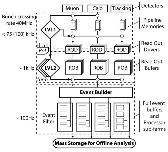
The design luminosity of the LHC ( $ \mathcal{L} $ = 10 $ ^{34} \Lum $) will give rise to 40 million bunch crossings occurring each second. It is expected that the total event rate after accounting for multiple interactions per bunch crossing will be of the order of 1 GHz, with a typical event size of the order of 1.5 MB. At the time of writing, technological limits placed a restriction on the speed of recording events to disk at the level of $ \approx $ 300 MB/s, thereby restricting the maximum rate of storing events to approximately 200 Hz. The ATLAS Trigger and Data aquisition (TDAQ) system is designed to facilitate the reduction of the event rate from the raw value of 1 GHz to 200 Hz and in doing so retain as many of the 'interesting' physics events (i.e. those relating to the goals of ATLAS outlined in the section The ATLAS Detector) as is possible. The Trigger system is based on three levels: Level 1, Level 2 and Event Filter, as illustrated in Figure 10. Level 2 and Event Filter together constitute what is termed the High Level Trigger (HLT) [17].

Figure 10: Overview of ATLAS Triggering system [18].

Signal and Background Processes

Signal Processes

The signal channel investigated in this study is a SM Higgs boson decaying to two Z bosons. As was shown in the section The Higgs Mechanism this decay mode is one of the dominant ones over a large range of high Higgs masses. The decay of the Z bosons considered is with one Z decaying to leptons and the other to neutrinos. Where one of the Z bosons decays to electrons(muons) this will subsequently be referred to as the electron(muon) channel (or $ \ztoee $ ( $ \ztomm $ ) channel). An individual channel is not considered for the case of the $ \tau $ lepton, but since $ \tau $ decays typically involve electrons/muons, in this sense they are included. From Figure 2, which gives a breakdown and branching ratios of the main Z decay modes, the main decays in this Higgs channel that include one Z decaying to leptons for triggering purposes are Z decays to leptons, leptons+jets and leptons+neutrinos. The decay to four leptons provides a signal which is the most easily identified in the detector, due to the presence of four high $ \pt $ leptons. However, it has the lowest BR, less than 0.1 $ \% $. In contrast the decay to leptons+jets has a much larger BR, $ \approx $ 14 $ \% $, but the presence of two jets makes it less easy to identify in the busy hadronic environment within ATLAS during data taking. The lepton+neutrino final state is perhaps a compromise between these. It has a BR in between the purely leptonic final state and the leptons+jets final state of $ \approx $ 4 $ \% $.

1: Here, and subsequently, lepton refers to either an electron or a muon.

The lepton+neutrino final state has missing energy coming from the two neutrinos in the final state, which provides a good way to discriminate over background. This was demonstrated in studies performed in this channel using the GF production mode [19] [20], which showed that particularly at high mass where, because of the Higgs decay products becoming more boosted with increasing mass, the large missing energy present in the signal gives good sensitivity. At lower Higgs mass however, the signal has much lower missing energy making discrimination against background more difficult.

This study takes a first dedicated look at the VBF production mode, in particular to see if the characteristics associated with the VBF topology in this decay channel may provide an improvement in sensitivity. However, focussing on the VBF production mode is also motivated as within the SM it is predicted to provide a different mechanism by which a Higgs type boson could be produced, compared to the cross section dominant GF mode, and so must be studied in order to verify if this prediction is correct. Further, the VBF production mechanism provides access to different couplings compared to the GF mode [21], which will need to be studied in order to cross check our understanding of the mechanism through which the weak-gauge boson and fermion masses are generated.

Figure 11: Comparison of Higgs boson (a) $ \pt $ and (b) $ \eta $ in vector boson fusion and gluon fusion produced truth signal events

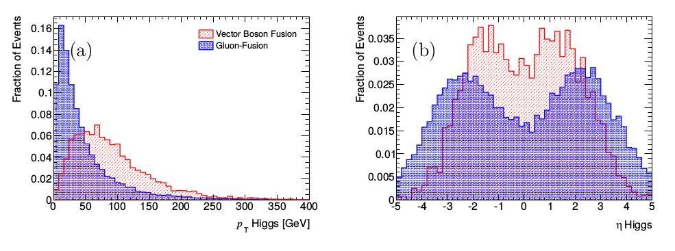
Typically the $ \pt $ of a Higgs boson produced in a VBF event is harder than that in a GF event, as can be seen in Figure 11, which uses Monte Carlo truth level (i.e. neglecting detector effects and allowing access to properties of underlying process) information in $ \htollnunu $ events. In addition it is more commonly in the central regions of the detector. These properties are a consequence of the Higgs boson recoiling off the typically forward tag-jets associated with the remnants of the VBF process (corresponding to the outgoing quarks produced in association with the Higgs boson as shown in Figure 6). Thus, the experimental signature of the signal in the VBF production mode is two hard isolated leptons, missing energy and tag-jets produced from the remnants of the VBF process.

Background Processes

The signal is expected to suffer from various SM background processes, which can be categorised into the following

top production via SM interactions
Single and di-boson production (with heavy quarks or jets)
QCD dijet and heavy quark production

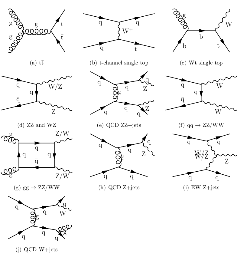
The production cross section for each of these backgrounds is orders of magnitude larger than the signal, requiring large background rejection in order for the signal to be detectable. Feynman diagrams of some of the backgrounds to this channel are shown in Figure 12. As an example of the kind of considerations made for each background, $ \toptop $ is discussed further in the following.

Figure 12: Feynman Diagrams of main backgrounds

Background example: Top Pair Production

The main decay modes of $ \toptop $ (Figure 12 a)) expected to contribute to the background to this analysis are where both of the Ws decay leptonically (lepton-lepton (ll) channel) and where one W decays leptonically and the other hadronically (lepton-hadron (lh) channel), making up $ \approx $ 6(34) $ \% $ of all $ \toptop $ decays respectively. The lepton-lepton channel final state contains two leptons, missing energy and two b-quark jets. This becomes a background when the detector fails to identify both of the b-quark jets either because they lie outside the acceptance of the tracker or because these jets don't pass the b-tagging criteria. The lepton-hadron channel becomes a background when one of the jets is misidentified as a lepton and the b-quark jets are not b-tagged. Because the top quarks recoil against each other when they are produced, the characteristics of the tag-jets in the signal may not provide much suppression of this background.

Phenomenology at hadron colliders and Monte Carlo simulation

The description of the Higgs signal and the explanation of its background processes earlier in this section do not take into account the fact that the LHC collides composite protons ($ A,B $). In order to model the interaction of composite protons at the energies produced by the LHC it is useful to consider the parton model in which the proton is made up of constituent partons ($ a,b $). In this model the interaction of individual partons leads to the production of other particles such as the Higgs boson ($ c $), the production cross section of which, $ d\sigma_{a+b\rightarrow c} $, can be found using the SM. In addition other remnants ($ Z $) will be produced. The calculation of the hadronic cross section ($ d\sigma_{A+B\rightarrow c+Z} $) however, must be calculated within the parton model according to $$ \begin{equation} d\sigma_{A+B\rightarrow c+Z} = \sum_{a,b} \int_{0}^{1} dx_{a} \int_{0}^{1} dx_{b} f^{a}_{A}(x_{a},Q^{2})f^{b}_{B}(x_{b},Q^{2})d\sigma_{a+b\rightarrow c} \label{BasicLHCProcess} \end{equation} $$ where the sum is over all processes (i.e. Feynman diagrams) contributing to the production of $ c $. $ f^{a}_{A} $ and $ f^{b}_{B} $ are called parton distribution functions (PDFs) and correspond to the probability to have a parton $ a $ with momentum fraction $ x_{a} $ within its parent proton $ A $ at energy scale $ Q $. These cannot be calculated from first principles but must be measured for example in deep inelastic scattering experiments. In this way the total hadronic cross section is composed of two parts, a perturbative short distance scale part and a non-perturbative long distance scale part. The procedure of separating the interaction like this is called factorization and the energy scale at which this is done is called the factorization scale. A diagram showing the different processes occurring when high energy protons collide is shown in Figure 13.

Figure 13: Phenomenological model of the interaction of a proton-proton collision at high energy scale. [22]

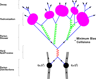
The interaction of the protons leading to, for example, the production of the Higgs boson represented by $ d\sigma_{A+B\rightarrow c+Z} $ is calculated within the parton model and corresponds to the hard sub-process. All other contributions to the final state not originating from the hard sub-process are called the underlying event. This includes initial state radiation (ISR) produced via emission from the incoming partons, interactions between the proton remnants (i.e. partons other than those in the hard interaction) and any final state radiation (FSR) from the final state particles. Because the final state partons carry colour charge they often radiate gluons, leading to production of quark anti-quark pairs. This gives rise to cascades of partons called parton showers. Once energetically favourable, the partons produced in such showers form colour neutral states in the process of hadronization. The decay products of these states are then subsequently measured in the detector. Understanding of parton showering and hadronization is achieved using dedicated models.

The most common technique to model physical processes is to use Monte Carlo methods. Monte Carlo methods use pseudo-random numbers to model particle interactions based on the underlying physical principles beyond the scope of this document. In particle physics this procedure is generally referred to as event generation and the program using the Monte Carlo methods is called the Monte Carlo generator. It allows the kinematics of any final state particles to be calculated given an input process and a set of initial starting conditions. The final state particles correspond to those that are stable in the sense that the distance they travel in the associated particle's proper lifetime is within a suitably large range. Some Monte Carlo generators simulate specific final states (called matrix element generators). This is typically done by summing over all relevant Feynman diagrams. An example is MC@NLO [23]. Other generators simulate non perturbative effects including hadronisation. An example is PYTHIA [24]. Details of the particles produced in the event generation are provided in the Monte Carlo $ truth $ information.

All Monte Carlo officially produced for the ATLAS Collaboration is produced within the ATHENA framework. This is a software framework which provides interfaces to all the generators used. In order to get a realistic picture of what we would expect to see in the detector when a particular process occurs, the interactions of the final state particles and the detector material are modelled. This procedure is done with the GEANT program and also performed in the ATHENA framework. Two approaches to this exist and are referred to as fast/full simulation respectively, depending on the level of detail at which the detector simulation is done.

Monte Carlo Samples

The Monte Carlo event samples used in this study were officially produced within the ATLAS Collaboration, using version 15.6.3 of the ATHENA framework. They were fully simulated using GEANT 4 and correspond to p-p collisions at $ \sqrt{s} $ = 7 $ \TeV $. The default samples used in this analysis do not model pile-up and are used to obtain the main results. This choice was made because of insufficient statistics in some of the pile-up samples for the backgrounds considered and because not all the processes considered were simulated taking pile-up into account. However, where possible the effect of pile-up was investigated. Where comparisons to pile-up Monte Carlo are made, this is explicitly stated and the pile-up Monte Carlo is referred to as such. The term Monte Carlo used without mention of pile-up corresponds to the non pile-up Monte Carlo. The pile-up samples considered were simulated with two interactions per bunch crossing. In the following the main properties of the simulated samples used will be discussed (signal and an example of one of the backgrounds).

Signal

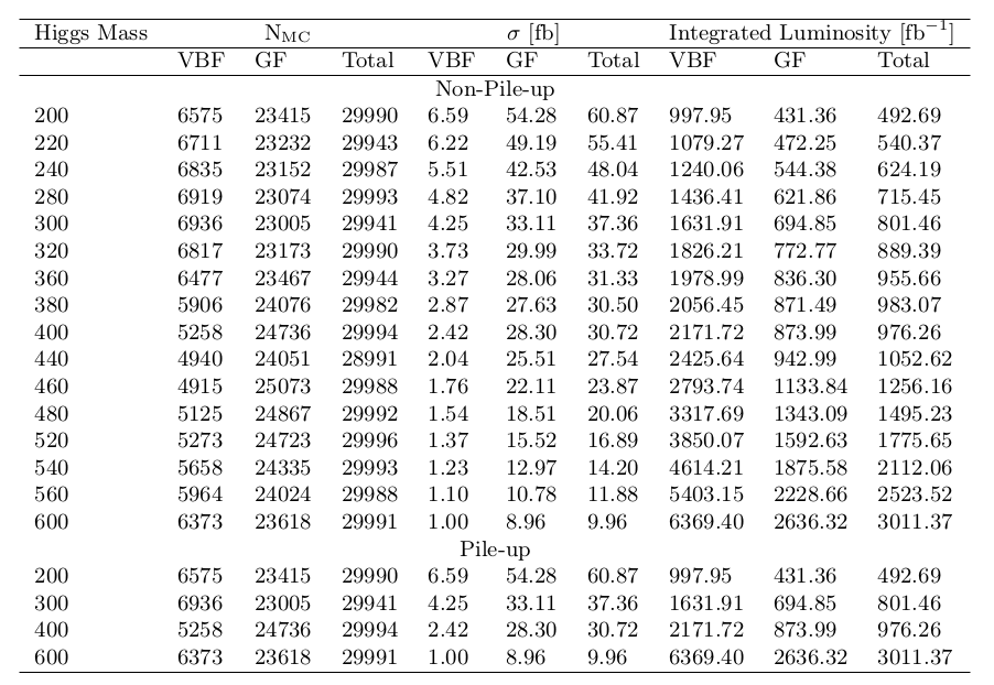
The signal samples used were generated with PYTHIA 6.421 [24]. Z decays to leptons included electrons, muons and taus in their corresponding branching fractions. ISR was modelled with PHOTOS [25] and the decay of tau leptons by TAUOLA [26]. The events include both VBF and GF contributions. The cross sections used are from [8], with GF quoted at NNLO and VBF at NLO. The analysis uses signal samples simulated for Higgs masses between $ \mH $ = 200-600 $ \Gcs $ in 20 $ \Gcs $ steps. The main properties of the signal samples used, including number of simulated events, cross section and the corresponding integrated luminosity are shown in Figure 14. A break-down of the VBF and GF components is shown. Separation of the samples into VBF and GF components was done using truth information. This was done by identifying the Higgs boson and then navigating backwards to identify if it was derived from gluons or quarks and so produced by GF or VBF. The identity of each particle was found using the PDG particle codes [4]. In order to verify that the separation of VBF and GF events was done correctly the fraction of VBF events obtained was compared to that produced in a statistically independent sample of $ \htollnunu $ produced with the same configuration options as the official ATLAS Monte Carlo. Agreement was found to within 1 $ \% $ for the range of mass samples tested ( $ \mH $ = 200-600 $ \Gcs $ in 100 $ \Gcs $ steps) indicating that the separation of VBF and GF was performed correctly.

Figure 14: Summary of signal Monte Carlo sample properties as a function of Higgs mass used in this analysis, including number of simulated events (N $ _{\mathrm{MC}} $ ), cross section ( $ \sigma $ [fb]) and corresponding integrated luminosity [ $ \fb $ ]. Included are the relative contributions from VBF and GF production mechanisms. The samples were generated with PYTHIA. Pile-up samples were simulated with two interactions per bunch crossing.

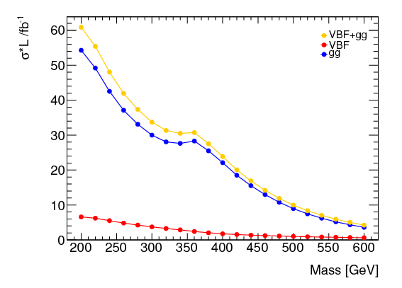
A comparison between VBF and GF cross sections at $ \sqrt{s} $ = 7 $ \TeV $ with varying Higgs mass is shown in Figure 15. The cross section is reduced by a factor six with increasing mass in the mass range investigated.

Figure 15: Comparison of predicted number of VBF and GF events produced at $ \sqrt{s} $ = 7 $ \TeV $ for 1 $ \fb $ as a function of Higgs mass.

Background example (Z+jets)

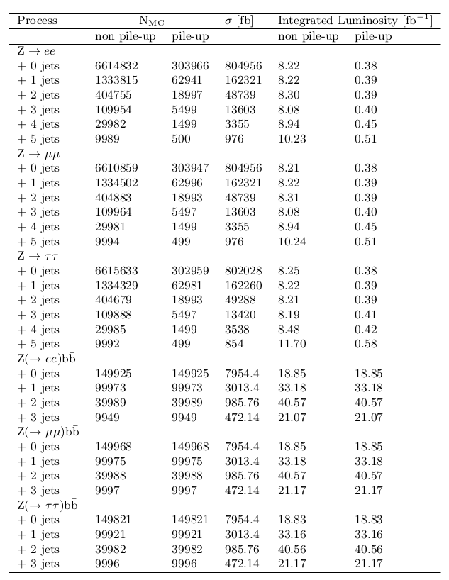
Z+jets samples were simulated with ALPGEN v2.13 [27] interfaced with HERWIG v6.510 [28] for modelling of parton showers and hadronization. The simulated samples include generated hard matrix elements for Z and Z $ \bb $ with additional numbers of partons in the final state: 0-5 partons for the Z samples and 0-3 partons for the Z $ \bb $ samples. In each case Z decays to $ ee,\mu\mu $ and $ \tau\tau $ are considered. The cross sections were taken from the generator prediction. A k-factor of 1.22 [13] is used to scale the LO generator cross section to NLO. Details of the Z+jets samples used are shown in Figure 16.

Figure 16: Summary of Z+jets Monte Carlo sample properties used in this analysis, including number of simulated events (N $ _{\mathrm{MC}} $ ), cross section ( $ \sigma $ [fb]) and corresponding integrated luminosity [ $ \fb $ ]. The samples were generated with ALPGEN interfaced with HERWIG.

p-p Collision Data

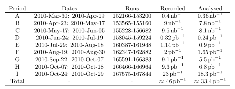
The real p-p collision data used in this study is from the ATLAS 2010 dataset, in which the LHC was operated at $ \sqrt{s} $ = 7 $ \TeV $ between 30 $ ^{th} $ Mar-29 $ ^{th} $ Oct 2010. During this time a total integrated luminosity of 48.8 $ \pb $ was delivered to ATLAS, of which 46.72 $ \pb $ was recorded. During the 2010 data taking period, the data taking sessions were divided up into periods, with each period made of a number of runs, each given a unique identifying number. A typical run involves a period of stable data taking whereby typically, beams are injected into the LHC, stable beams are declared and data taking is maintained until beams are dumped or lost. The data in 2010 is composed of periods A to I. Each run is composed of fixed luminosity intervals called lumi-blocks. Within ATLAS, for each lumi-block a set of indicators called data quality flags are used to identify beam and detector conditions. This information is exercised by physics analysers who use 'Good Run Lists' (GRLs) to specify which quality flags they require to be passed for their analysis. For the purpose of this study, only runs passing certain quality requirements/flags were taken into account. In particular the following flags were required to be passed:

ATLGL- requires that the run has been evaluated by the data quality group.
LUMI- requires luminosity and forward detectors are operational and luminosity is correctly calculated.
ATLSOL, ATLTOR- requires the currents in the solenoid and toroid magnets to be stable.
L1CTP, L1CAL, L1MUB, L1MUE- requires the Level 1 Central Trigger Processor, calorimeter trigger and barrel/end cap muon triggers are performing with a good efficiency and there are no timing, synchronisation or data flow problems.
cp_eg_electron_barrel, cp_eg_electron_endcap, cp_mu_mstaco, cp_mu_mmuidcb, cp_jet_jetb, cp_jet_jetea, cp_jet_jetec- are required to allow measurement of electrons, muons and jets. cp_met_metcalo, cp_met_metmuon- are required for $ \etmiss $ measurement (the latter was not required for periods A-C since this flag was not present).
cp_tracking- requires inner detector in good working order.
cp_btag_life- requires detector sub-systems required for b-tagging measurements are operable (not required for periods A-C since this flag was not present).

This was implemented by applying a GRL, based on that detailed in [19]. The 2010 data was analysed using the recommended physics containers, corresponding to datasets for each trigger stream used. In order to maximise the amount of collected data different trigger requirements were made according to the running conditions in each run. Using this setup a total of 33.4 $ \pb $ of the 2010 data was analysed. A breakdown of how much luminosity was analysed per period is shown in Figure 17.

Figure 17: Details of the data used in this analysis.

Physics Objects

In essense, the different parts of the detector are designed to detect different physics objects (jets, leptons and neutrinos). However, this is done through reconstruction and identification methods, as the detector components themselves, more often than not through some physical process (often the particle in question reacting in some way with a particular component of the detector), measure electrical raw signals. The aim of the "reconstruction" of physics objects is to as accurately as possible reconstruct, on an event by event basis, the truth particles within the Monte Carlo simulation and the actual particles produced in real proton-proton collisions from the raw signals from the sub-detectors. Within ATLAS, this procedure is performed within the ATHENA framework (version 15.6.13 was used in this study). Because of limitations in the measurement accuracy of the detector sub-systems or approximations in the algorithms used to perform the reconstruction process, a 100 $ \% $ accurate reconstruction is not achievable. For example a particle may be reconstructed as the wrong type or not be detected at all. In order to quantify the level of this inconsistency the definitions of reconstruction efficiency and misidentification rate are commonly used. The reconstruction efficiency $ \epsilon $ of a particle represents the fraction of true particles (in this study corresponding to the Monte Carlo truth particles) that are correctly reconstructed as that type of physics object. In this case the reconstruction efficiency can be expressed as shown in Eqn. \eqref{eqn_identificationEffic}, $$ \begin{equation} \epsilon = \frac{N^{matched}}{N^{all}} \label{eqn_identificationEffic} \end{equation} $$

where $ N^{all} $ is the total number of Monte Carlo truth particles and $ N^{matched} $ is the number of these that $ match $ a reconstructed object of the same type.

In order to quantify the rate at which a particle is mis-identified, the mis-identification rate ($ \chi $) shown in Eqn. \eqref{eqn_identificationFakeRate} is defined as the number of reconstructed objects not matched to a truth particle of the same type ($ N^{not-matched} $) divided by the total number of reconstructed objects ($ N^{all-reconstructed} $). $$ \begin{equation} \chi = \frac{N^{not-matched}}{N^{all-reconstructed}} \label{eqn_identificationFakeRate} \end{equation} $$

The signal within this analysis contains electrons, muons and jets and so it is particularly important that these objects are well reconstructed. To this end, the efficiency and mis-identification rates in the signal have been studied and compared to the performance of some of the main backgrounds in this analysis. The matching criteria used is a geometrical matching requiring the $ \Delta R $ between the truth particle and reconstructed object to be less than 0.02 for electrons and muons and 0.1 for jets.

First, as an example, the methods used to reconstruct electrons are discussed. Then any specific requirements for the objects used in the analysis are defined and examples of the performance of reconstruction of the various physics objects is summarised.

Electrons

The high rates expected from the vast QCD background at the LHC will make it difficult to correctly reconstruct and identify electrons over the broad $ \pt $ range they will be produced in by the physics channels of interest. Within the $ \pt $ range 20-50 $ \Gc $, the rate of production of isolated electrons compared to QCD jets will be below 10 $ ^{-5} $. Although this effect is reduced at higher energy, high jet-rejection is required.

Electron Reconstruction

Electrons are reconstructed using both calorimeter and inner detector information in ATLAS. There are two main algorithms for reconstruction within the inner detector acceptance ($ |\eta| < $ 2.5). The EGAMMA algorithm is designed to reconstruct high $ \et $ isolated electrons. It is seeded by energy deposits in cells in the electromagnetic calorimeter and then searches for a matching track in the inner detector. The $ softe $ algorithm is optimized to reconstruct soft (low $ \pt $) electrons and is seeded by an inner detector track. It then searches for a matching EM cluster in the electromagnetic calorimeter. The electrons in the H $ \rightarrow $ ZZ $ \rightarrow \ell\ell\nu\nu $ signal are expected to be energetic so only electrons reconstructed with the EGAMMA algorithm are used and are discussed in the following.

Electron Identification

After a candidate electron has been reconstructed, an electron identification procedure is applied to establish its reconstruction quality. Currently the default identification procedure applies a series of cuts related to shower shape, tracking and cluster-track matching variables (which are optimized according to $ \et $ and $ \eta $). Three standard electron definitions are used: $ Loose $, $ Medium $ and $ Tight $, each corresponding to an increasingly selective set of cuts, whereby each definition includes the cuts of the looser definitions.

Electrons used in this analysis

Electrons used in this analysis are reconstructed with the standard EGAMMA algorithm and are required to have an electron track within the acceptance of the tracker and electromagnetic calorimeter and electron energy measured in the calorimeter $ \et $ > 20 $ \GeV $. Electrons are required to pass the $ Robust $ - $ Medium $ identification cuts. $ Robust $ - $ Medium $ electrons correspond to $ Medium $ electrons, with a few changes that were introduced by the $ e \gamma $ performance group in order to maintain the robustness of electron identification by accounting for discrepancies between Monte Carlo and 2010 data. In particular the electron shower shapes were shown to be wider in data compared to Monte Carlo and as such cuts on $ R_{\eta} $ and $ w_{\eta2} $ are loosened. Further the hadronic leakage cut is modified due to a change in the modelling of the hadronic calorimeter noise (in early data it is modelled with a wider double gaussian). Any reference to electrons now refers to the $ Robust $ - $ Medium $ definition [29].

During the 2010 data taking period a number of cells in the electromagnetic calorimeter were lost because of problems in its readout electronics. In order to account for this effect, which is not taken into account in the Monte Carlo samples used, the (OTX) procedure to remove any electrons in the regions around the lost cells is implemented. In order to identify the lost cells the database corresponding to that at the end of the 2010 data taking period (from Run 167521) is used.

A number of additional corrections [30] are applied to the data and Monte Carlo which have been recommended by the $ e \gamma $ performance group in order to improve the agreement between them. The energy scale of electrons in data is corrected by the expression $ E_{Corrected} = E_{Original}/(1+scale) $ where $ scale $ is equal to -0.0096 if $ |\eta_{cluster}| $ < 1.4 and 0.0189 for 1.4 < $ |\eta_{cluster}| $ < 2.5, where $ \eta_{cluster} $ is the electron cluster $ \eta $. In order to maximise the reconstruction efficiency electrons within the crack region between 1.37 < $ |\eta| $ < 1.52 are used. For the $ \mH $ = 200 $ \Gcs $ signal this was shown to provide an increase in VBF statistics by approximately 8 $ \% $. The energy of electrons in the crack is scaled by 5 $ \% $ in the data and 3 $ \% $ in the Monte Carlo. In addition, the identification efficiency of electrons measured in $ \ztoee $ and $ \W \rightarrow e \nu $ suggests that for $ Robust $ - $ Medium $ electrons Monte Carlo overestimates the efficiency. This is corrected for by weighting the Monte Carlo with $ \eta $ dependent scale factors [31].

Overall performance of electron identification with corrections

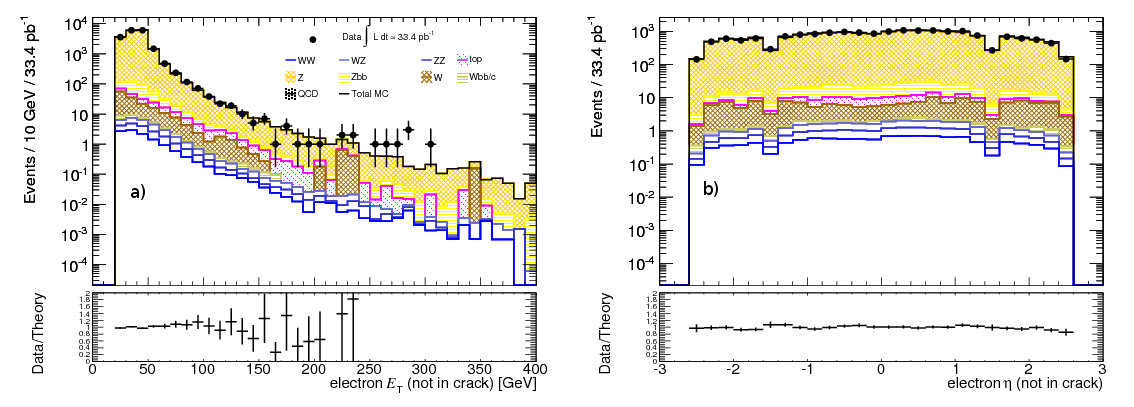
The efficiency of the electron selection used in this analysis for the VBF $ \mH $ = 200 $ \Gcs $ signal sample and two different backgrounds which are expected to be a source of relatively isolated electrons ( $ \ztoee $ ) and non-isolated electrons ($ \toptop $) was investigated. The efficiency is measured by comparing reconstructed electrons with respect to Monte Carlo truth level electrons with $ \et $ > 20 $ \GeV $ and $ |\eta| < $ 2.5, using a matching criteria of $ \Delta R < $ 0.02. As expected the source of isolated electrons $ \ztoee $ has the largest efficiency for the EGAMMA algorithm. However, it is promising that the signal shows a larger efficiency compared to the source of relatively non-isolated electrons, $ \toptop $, by nearly 20 $ \% $. Furthermore, requiring the $ Robust $ - $ Medium $ identification, the efficiency for the signal and the $ \ztoee $ reduces by approximately 10 $ \% $, whereas for the $ \toptop $ this is closer to 20 $ \% $. Beyond this level, the cuts applied have a similar effect on each sample as expected.

A comparison of data and Monte Carlo of some basic electron variables including electron $ \et $ and $ \eta $ (without crack electrons) is shown in Figure 18. As with all subsequent object distributions in this section, the plot shows the total background Monte Carlo distribution, represented by the total MC line together with the contribution of each background considered.The dataset analysed is added and shown by the circular markers. These distributions are made with the lepton requirements detailed in the section Lepton Selection. Good agreement is found between data and Monte Carlo for non-crack electrons while despite the corrections applied for crack electrons, they are underestimated at low $ \et $ in the Monte Carlo.

The electron identification efficiency and mis-identification rates as a function of electron $ \et $ and $ |\eta| $ were also investigated. Included is a comparison of the $ \mH $ = 200 $ \Gcs $ signal, $ \ztoee $ and $ \toptop $. Reconstructed electrons are required to pass the selection criteria outlined previously while Monte Carlo truth electrons must have $ |\eta| < $ 2.5 and $ \et > $ 22(18) $ \GeV $ for the efficiency(mis-identification) calculation respectively, in order to account for resolution effects. Electron efficiencies are observed to increase with $ \et $. With $ \eta $ the reconstruction efficiency is fairly constant although between 1.37 < $ |\eta| $ < 1.52 it drops because of the electromagnetic barrel-end-cap transition. At higher $ \eta $ reconstruction efficiency worsens due to poorer tracking performance in the forward regions. Comparing the different samples included, it is seen that the source of non-isolated electrons $ \toptop $ shows a lower reconstruction efficiency than the signal and the source of isolated electrons a higher efficiency. This trend is seen as a function of $ \et $ and $ |\eta| $.

The VBF component of the signal shows a larger mis-identification rate compared to the GF component. This is attributed to the VBF component being a source of less isolated electrons. For the same reason, the mis-identification rate for $ \toptop $ is larger than that for $ \ztoee $. As expected the mis-identification rates reduce with $ \et $ due to the higher identification efficiency with increasing $ \et $. The trend in $ |\eta| $ is approximately constant but is reduced in the crack region because of decreased efficiency.

Figure 18: Comparison of data and Monte Carlo a) $ \et $ and b) $ \eta $ distributions for electrons (not in crack) used in this analysis.

Muons

Muons are reconstructed from the tracks they produce in the Inner Detector and Muon Spectrometer. Three different types of muon object can be reconstructed depending on the availability of information from these detector sub-systems. Standalone muons are reconstructed from a Muon Spectrometer track over its acceptance ($ |\eta| < $ 2.7). Combined Muons are reconstructed over the acceptance of the Inner Detector ($ |\eta| < $ 2.5), by matching a standalone muon to an Inner Detector track and combining the measurements. Segment tagged muons are reconstructed from an Inner Detector track matched to a short Muon Spectrometer track, typically within one innermost station (called a segment).

Muons used in this analysis

In this study, combined and segment tagged muons from the STACO family are used. Muons must have a $ \pt > $ 20 $ \Gc $ and $ |\eta| < $ 2.5. Muon tracks are required to be isolated by requiring the sum of the momenta of all tracks with $ \pt > $ 1 $ \Gc $ in a cone $ \Delta R $ = 0.2 around the muon to be less than 0.8 $ \Gc $. Additional requirements are made on the muon quality subject to recommendations from the muon combined performance group guidelines [32] which are largely to protect against muon solenoid - inner detector track mis-matching. As such identified muons are required to have traversed all the inner detectors sub-detectors, depositing $ \geq $ 1 pixel hits, $ \geq $ 6 SCT hits on the muon track. Within the acceptance of the TRT, hits are required as follows. Defining n $ _{TRThits} $ as the number of TRT hits on the muon track and n $ _{TRToutliers} $ the number of TRT outliers on the muon track, for $ \eta < $ 1.9 the sum of n $ _{TRThits} $ and n $ _{TRToutliers} $ (n) is required to be greater than 5 and n $ _{TRToutliers} $ < 0.9 n. For $ \eta $ > 1.9, if n > 5, then it is required that n $ _{TRToutliers} $ < 0.9 n. Additionally for combined muons $ \chi^{2}_{match} $ is required to be less than 150 and for tracks with muon spectrometer transverse momentum $ \pt $ (MS) < 50 $ \Gc $ the difference between the extrapolated momentum in the muon spectrometer $ p $ (MS extrap) and the momentum in the inner detector $ p $ (ID) must be greater than 0.4 $ p $ (ID). In order to suppress cosmics the distance of closest approach relative to the primary vertex (the transverse impact parameter, d0) is required to be less than 1 mm and the absolute value relative to the $ z $ vertex at the beam-line (Z0) is required to be less than 1 cm. A number of additional corrections are applied to muons in the Monte Carlo following the recommendations from the muon performance group. The performance of the transverse momentum scale and resolution for combined muons was measured in the data using the di-muon mass distribution in $ \ztomm $ decays [33]. It was found that the muon energy scale is reasonably well described and so no correction is applied. However, it was shown that the resolution in the data is poorer compared to that in the Monte Carlo. The difference is used to define smearing factors for the Monte Carlo for the inner detector and muon spectrometer momentum components. If both the inner detector and muon spectrometer components were measured, the overall transverse momentum of the combined muon is found by weighting the components by their relative resolution. For cases where no measurement was made in the muon spectrometer (inner detector) the muon $ \pt $ is taken to be the smeared inner detector (muon spectrometer) $ \pt $. This procedure was done using the official code provided by the muon performance group. In [34] it is shown that for combined and segment tagged muons, the muon efficiency in the simulation and the data are well matched. Therefore no correction is applied.

Overall performance of muon identification with corrections

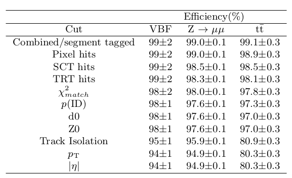
The efficiency of the muon selection used in this analysis for the $ \mH $ = 200 $ \Gcs $ signal sample and two different backgrounds which are expected to be a source of relatively isolated ( $ \ztomm $ ) and non-isolated ($ \toptop $) muons are shown in Figure 19. The efficiency is measured by comparing reconstructed muons with respect to Monte Carlo truth level muons with $ \pt $ > 20 $ \Gc $ and $ |\eta| $ < 2.5, using a geometrical matching criteria of dR < 0.02. The efficiency achieved in the signal is close to that in $ \ztomm $ and similar to the value quoted in [34] of 97 $ \% $. The performance for $ \toptop $ is reduced by a further 10 $ \% $ and is shown to be due to the track isolation cut, due to the presence of non-isolated muons in this sample.

Figure 19: Efficiency of Muon selection cuts. Efficiencies are shown for $ \mH $ = 200 $ \Gcs $ VBF $ \htollnunu $ signal sample, $ \ztomm $ and $ \toptop $. Efficiencies are calculated by comparison of Monte Carlo truth and reconstructed muons.

As was done for electrons, a comparison of data and the Monte Carlo prediction for some of the main muon variables was performed. The distributions were made using the lepton requirements detailed in the section Lepton Selection. A good level of agreement was found.

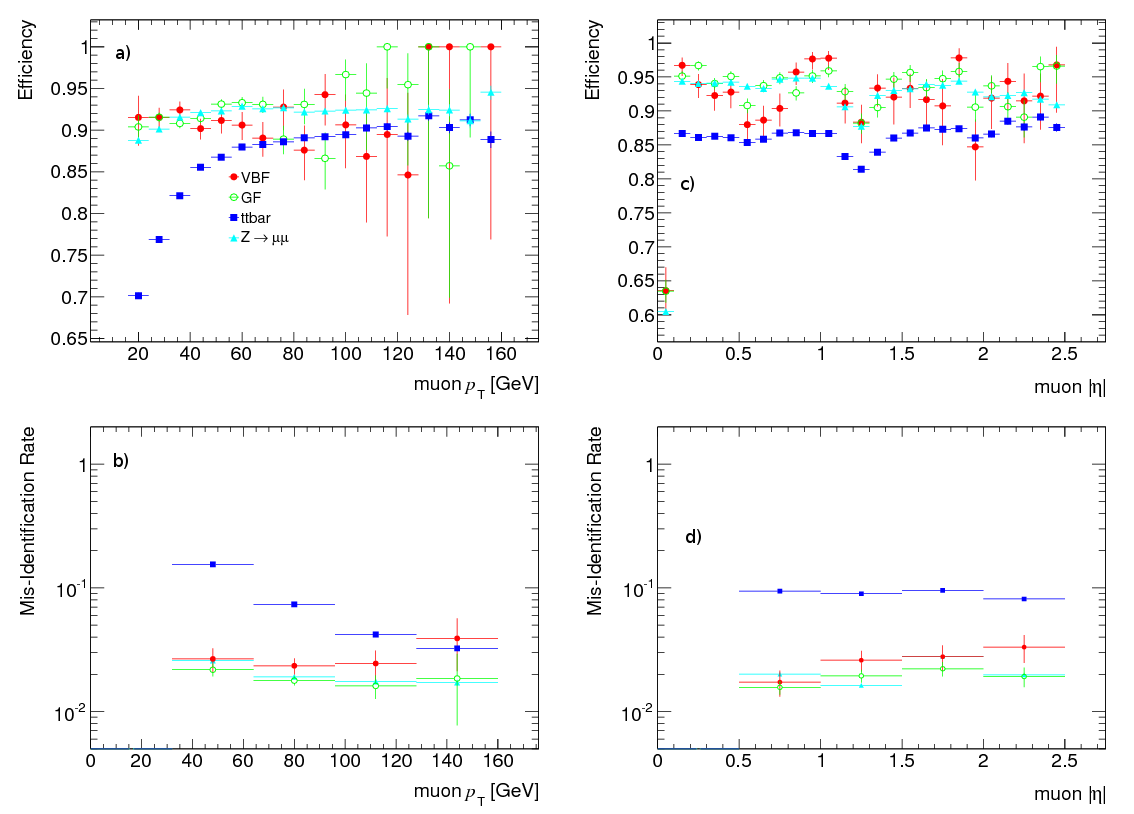
The muon identification efficiency and mis-identification rates for the muon selection adopted in this analysis as a function of muon $ \pt $ and $ |\eta| $ are shown in Figure 20. Included is a comparison of the $ \mH $ = 200 $ \Gcs $ signal, $ \ztomm $ and $ \toptop $ samples. Reconstructed muons must satisfy the muon selection detailed previously and Monte Carlo truth muons $ |\eta| < $ 2.5 and $ \pt > $ 22(18) $ \Gc $ for the efficiency(mis-identification) calculation. Muon efficiencies are observed to increase with $ \pt $ until 60 $ \Gc $ at which point there is a plateau region where they remain approximately constant. With $ \eta $ the reconstruction efficiency rises quickly from low $ \eta $ where the detector acceptance is poor due to the detector support structure. Efficiency is also degraded in the transition region between 1.1 < $ |\eta| $ < 1.7 where there are fewer muon stations. Muon mis-identification rates are highest for the $ \toptop $ due to the presence of non-isolated muons making reconstruction more difficult. At the other extreme, $ \ztomm $ exhibits the lowest mis-identification rate. Although higher than in the GF component of the signal, the mis-identification rate of the VBF signal is lower than that in $ \toptop $. These findings indicate that adopting the selection described, muons can be identified efficiently in the signal and with fewer mistakes compared to a major expected background, $ \toptop $.

Figure 20: Muon reconstruction efficiency (upper plots) and mis-identification rate (lower plots) as a function of (a,b) $ \pt $ and (c,d) $ |\eta| $ for VBF signal (filled circles), GF signal (open circles), $ \toptop $ (filled squares) and $ \ztomm $ (filled triangles) after the pre-selection of muons. Signal components correspond to the $ \mH $ = 200 $ \Gcs $ sample.

Jets

Jets are collimated hadrons produced by energetic partons. They deposit energy in the electromagnetic and hadronic calorimeters and if charged, tracks in the Inner Detector. Jets are reconstructed using calorimeter information, over its full acceptance ($ |\eta| < $ 4.9). They are reconstructed using jet-finding algorithms, of which there are many examples, but each of which reconstructs jets from input objects by combining their four momenta. The input to jet-finding algorithms does not have to be derived from the calorimeter (giving calorimeter jets), tracks or particles from an event generator are possible inputs. In order to reconstruct calorimeter jets, the calorimeter cells are combined into larger objects called calorimeter towers or topological cell clusters, which form the input to the jet-finding algorithms.

Jets used in this analysis

The jets used in this analysis are reconstructed using the anti-$ k_{T} $ algorithm with a distance parameter of 0.4, calibrated using global calibration. Topological clusters are used for the jet algorithm input. The energy scale of jets is corrected from the electromagnetic scale to the hadronic scale using the recommended $ \pt $ and $ \eta $ dependent Jet Energy Scale. This was derived from Monte Carlo but verified with data, and as such is expected to give a more accurate calibration at the time of writing. Jets must have a $ \pt > $ 20 $ \Gc $ and $ |\eta| < $ 4.5. In order to suppress the contribution of a jet in other than the p-p collision from which it originated, at least 75 $ \% $ of any tracks originating from the jet are required to be associated with the primary vertex of the given p-p collision. This is achieved by requiring that the jets have a Jet Vertex fraction $ |JVF| $ > 0.75. In this way the effect of in-time pile-up causing multiple p-p collisions to occur within the same bunch crossing can be reduced.

Overall performance of jet identification with corrections

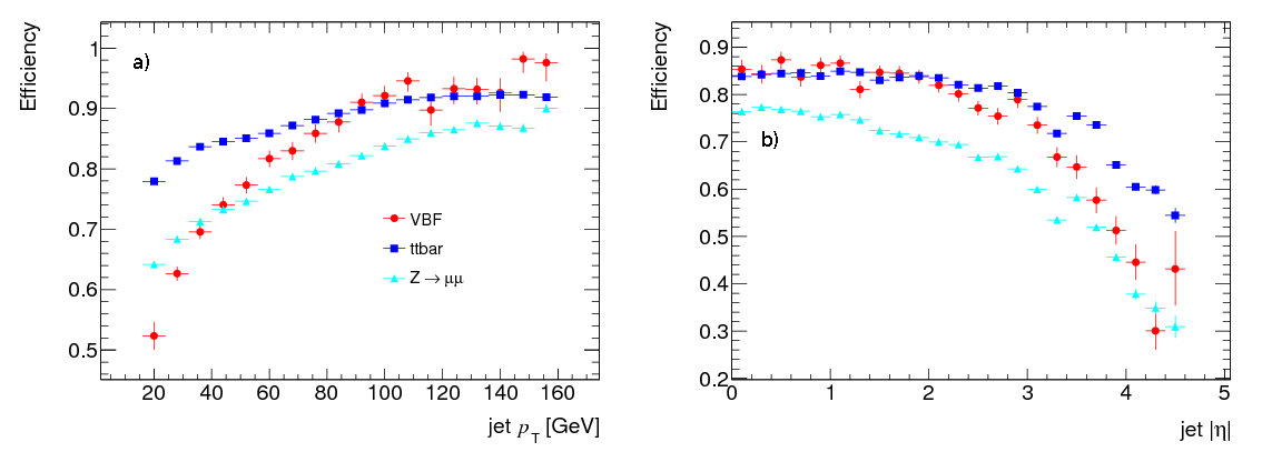
The reconstruction efficiency of jets used in this analysis as a function of $ \pt $ and $ |\eta| $ is shown in Figure 21 for the $ \mH $ = 200 $ \Gcs $ signal, $ \ztomm $ +jets and $ \toptop $ samples. The performance of jet reconstruction in the VBF signal appears to be slightly worse than in $ \toptop $ at low jet $ \pt $ and large $ |\eta| $. In comparison, the performance in $ \ztomm $ +jets is lower compared to that in the signal across the entire $ |\eta| $ range investigated. Overall, for the signal, a jet reconstruction efficiency of over 60 $ \% $ is maintained for jet $ \pt > $ 30 $ \Gc $ and $ |\eta| < $ 3.5.

Within ATLAS there are a number of b-tagging algorithms to differentiate the decay of a b-hadron from that containing only light quarks. In this analysis this is particularly important in order to suppress backgrounds such as those with a top quark decay. The b-tagging algorithms use the fact that hadrons with a b quark have a much larger lifetime giving a pronounced decay length c $ \tau\approx $ 450 $ \mu $ m compared to light quark hadrons. They are identified either by using reconstructed secondary vertices from the tracks within a jet or by combining the distance of closest approach to the primary vertex of all tracks in the jet. Within this analysis, decays of b hadrons are identified using the secondary vertex based algorithm SV0 [35]. A jet is called a b-jet if its lifetime-signed decay length significance (b-tag weight) is greater than 5.72 (this follows [36]).

A series of cuts are applied to ensure that the jets used are free from electromagnetic coherent noise bursts, calorimeter spikes and cosmics/ beam background. They follow the recommendation of the Jet $ \etmiss $ group [37] and as such any jet in the data which fails one of the $ loose $ criteria is rejected and not considered further in the analysis. Any event with a $ bad $ jet with $ \pt $ > 20 $ \Gc $ is then rejected. This selection is only implemented on data as the distributions relating to the selections are not well modelled in simulation.

Figure 21: Jet reconstruction efficiency as a function of a) $ \pt $ and b) $ |\eta| $ for VBF component of signal (filled circles), $ \toptop $ (filled squares) and $ \ztomm $ +jets (filled triangles) after the preselection of jets. The signal sample corresponds to $ \mH $ = 200 $ \Gcs $.

Missing Transverse Energy ($ \etmiss $)

Typically weakly interacting particles such as neutrinos will traverse the entire detector volume without leaving any measurable signal. As such they have to be measured indirectly through the imbalance of observed transverse momentum they cause which is commonly expressed through the quantity $ \etmiss $. Reconstruction of $ \etmiss $ in ATLAS [38] [39] is in essence done by summation of all energy deposits in the calorimeter cells and muon tracks. However it is complicated as there are many processes apart from the hard scattering process such as the underlying event, multiple interactions, pile-up and coherent electronics noise, which give rise to such energy deposits and muon tracks. To achieve an accurate measurement of $ \et $ and therefore $ \etmiss $, each component must be correctly calibrated and corrections for energy loss in non-active material have to be accounted for. It is further made difficult due to fake $ \etmiss $ coming from noisy/dead calorimeter cells, badly reconstructed/fake muons and acceptance effects due to lack of detector coverage.

Missing Transverse Energy used in this analysis

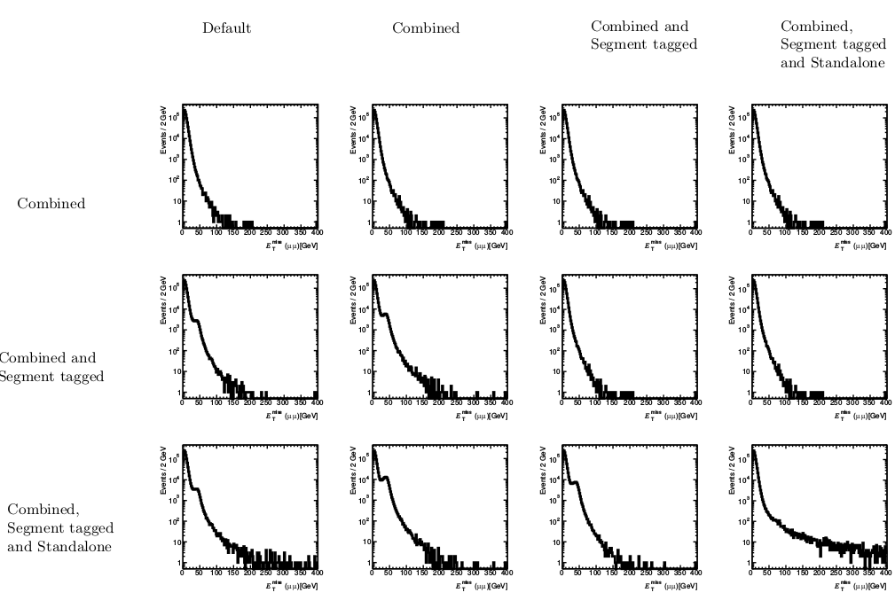
The definition of $ \etmiss $ used in this analysis follows what at the time of writing was currently recommended. It is called MET $ _{LocHadTopo} $ and uses the cell-based approach using TopoClusters within $ |\eta| < $ 4.5. The calorimeter cell energy is calibrated using weights from local hadron calibration of TopoClusters. As recommended, in events where there are muons passing the muon selection criteria outlined, the muon terms ( $ \etmissmuon $ ) in the $ \etmiss $ definition are removed and replaced explicitly with the muons found in the event, in order to avoid double counting. The motivation for this is shown in Figure 22, where the $ \etmiss $ distribution in $ \ztomm $ events is presented when different types of muons are selected (rows) and different types of muon are used in order to correct the $ \etmiss $ distribution (columns). The default $ \etmiss $ variable is plotted in the left-most column. Combined and segment tagged muons are required to have a $ \pt $ > 20 $ \Gc $ and $ |\eta| < $ 2.5 while standalone muons are required to have $ \pt $ > 20 $ \Gc $ and $ |\eta| < $ 2.7. When combined and segment tagged muons are used in the selection (like in this study) if no replacement of the muon terms is made in the $ \etmiss $ expression, then a bump around 50 $ \GeV $ appears in the $ \etmiss $ distribution. This problem is only resolved when the muon terms are replaced explicitly with the combined and segment tagged muons in the event.

Figure 22: $ \etmiss $ in $ \ztomm $ events. The rows represent the different types of muons considered. The leftmost column shows the default $ \etmiss $ distribution. Moving from left to right in the columns, shows the effect of replacing the $ \etmissmuon $ term with different types of muons.

Overlap Removal

Reconstruction of jets is based on information from the calorimeter only. As a consequence of this energy depositions produced by electrons and photons can be reconstructed as jets. To avoid using such jets in the analysis which are actually electrons, jets which overlap within $ \Delta R $ < 0.4 with a electron satisfying the electron quality requirements detailed are removed. Likewise, any jet within $ \Delta R < $ 0.4 of a muon satisfying the requirements outlined is removed. Priority is given to muons over electrons and as such any electron within $ \Delta R < $ 0.2 of a muon is removed.

Feature Selection

In this section the cut-based selection used for the search for the SM Higgs boson in the $ \htollnunu $ channel produced by VBF is detailed. First the event pre-selection cuts are discussed and motivated. Subsequently discriminating variables associated with the Higgs decay products are described and a baseline set of cuts on these variables discussed. Next the variables useful to discriminate between signal and background that are associated to the VBF remnants are described. In each case the results of the baseline selections are summarised. In addition the effect of pile-up on each variable of interest is investigated and comparisons between data and Monte Carlo are made in order to ensure the variables used are well understood. For samples with an insufficient number of Monte Carlo events an attempt is made to estimate the contribution of these backgrounds.

Preselection

The following outlines the pre-selection cuts used. Half of the available Monte Carlo events is used so that cuts can be optimized on an independent sample. Firstly, at least one primary vertex with at least three associated tracks ($ \pt > $ 150 $ \Mc $) is required.

In order to be able to record signal events, this analysis relies on two single lepton triggers, designed to exploit the high $ \pt $ leptons in the signal. In the Monte Carlo samples used in this study, not all triggers used on the data were available in the ATHENA release used. In the electron channel ($ \ztoee $) the L1_EM14 trigger is used while in the muon channel ($ \ztomm $) the Event Filter chain EF_mu10_MG is used (same triggers used in pile-up Monte Carlo). These require an electron with transverse energy greater than 14 $ \GeV $ and a muon with a transverse momentum of 10 $ \Gc $ respectively. These triggers were shown to have comparable efficiency to those used in the data [19].

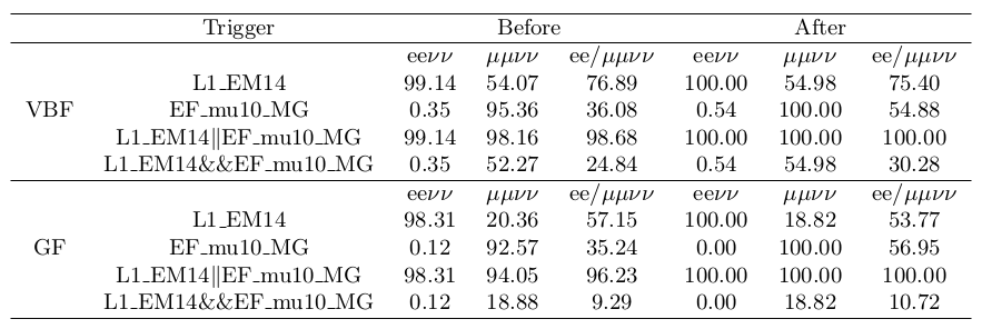
A comparison of the trigger efficiency of the VBF component of the signal compared to the GF signal, using the $ \mH $ = 200 $ \Gcs $ signal sample, for each combination of triggers used on the Monte Carlo before and after the offline selection of the lepton candidates is shown in Figure 23. The performance of the individual triggers is shown to be above 90 $ \% $ in both the electron and muon channels for each signal component before the lepton selection. After the selection of lepton candidates this rises to 100 $ \% $ in each case. This indicates that the use of single lepton triggers provides adequate performance for triggering both components of the signal. A certain level of overlap is shown to exist between triggers and channels although this appears to be much reduced with the muon trigger, where the muon trigger fires in the electron channel typically less than 1 $ \% $ of the time. In contrast, for the electron trigger this value is closer to 50 $ \% $, caused by the looser nature of the electron trigger employed.

Within the pre-selection cuts as expected the vertex cut has a small but similar effect on all samples, typically reducing sample statistics by less than 1 $ \% $. For all samples considered the electron trigger is more efficient than the muon trigger. This is expected because the electron trigger is a Level 1 trigger whereas the muon trigger is an Event Filter trigger and therefore places much stricter requirements on the muons being triggered. Typically, the trigger efficiency for samples with isolated electrons(muons) is around 60(40) $ \% $ respectively. For samples with non-isolated leptons, the triggering efficiencies are much lower at less than 30(20) $ \% $ for electron(muons).

Figure 23: Trigger selection efficiencies ($ \% $) for different combinations of electron (L1_EM14) and muon (EF_mu10_MG) triggers for VBF (upper section) and GF only (lower section) components of the $ \mH $ = 200 $ \Gcs \htollnunu $ signal sample. Efficiencies are given for both the generated sample and the sub-sample containing two reconstructed electrons or muons passing the selection requirements. In each case this is broken down into H $ \rightarrow $ ee $ \nu\nu $ , $ \mu\mu\nu\nu $ ,ee $ +\mu\mu\nu\nu $ events using truth information.

Selection based on Higgs decay products

In the following the variables that provide good discrimination between signal and background that are related to the decay products of the Higgs boson are motivated and a baseline selection adopted. This selection is based on the work performed in an analysis targeting the GF component of the signal [19] [20], which was used for validation purposes. Cut variables identified in this work were investigated in the context of the VBF signal and cuts changed appropriately. Comparisons are made with data and pile-up Monte Carlo reweighted to show similar levels of pile-up as that in the data analysed. By this procedure any regions where there are discrepancies between the nominal non-pile-up Monte Carlo and/or the data and pile-up reweighted Monte Carlo are avoided in order to try to maximise robustness of the analysis.

In order to correct the pile-up Monte Carlo to reflect the level of pile-up seen in the data an event reweighting procedure is performed on the pile-up Monte Carlo samples. In this procedure, the number of primary vertices in the event with three or more tracks is plotted after the di-lepton mass window cut (which is motivated later in this section) for the total background using the pile-up Monte Carlo and the data [19]. With each distribution normalised to unity, event weights as a function of the number of primary vertices were derived by taking the ratio of data over Monte Carlo for each bin. A much improved agreement between data and pile-up Monte Carlo is achieved when this Monte Carlo has been reweighted.

Lepton Selection

Typically backgrounds with no real leptons coming from the hard process will produce fake leptons which have a softer $ \pt $ distribution. For backgrounds with real leptons the $ \pt $ hardness is not much different to the signal. In this sense the lepton $ \pt $ cut serves to act to make sure the leptons selected are of good quality. This will allow further suppression of backgrounds without real leptons such as QCD. As detailed in the section Electrons used in this analysis, electrons used in this study are required to have $ \et > $ 20 $ \GeV $ and muons are required to have $ \pt > $ 20 $ \Gc $.

The presence of two leptons from the leptonically decaying Z boson in the signal topology allows for efficient rejection of backgrounds without isolated leptons, namely QCD. The distributions of the electron and muon multiplicities for events with either two electrons (corresponding to $ \ztoee $ in signal) or two muons ( $ \ztomm $ in signal) satisfying the criteria outlined in the section Physics Objects are shown in Figure 24. By requiring exactly two electrons or two muons and no leptons of any other type allows for rejection of some background, particularly the di-boson background. From now on $ \ztoee $ will be used to refer to events with exactly two electrons and no muons and $ \ztomm $ to events with exactly two muons. In the case of $ \ztomm $ in order to maintain good muon identification, at least one muon is required to be combined. It is possible the contamination of electrons in the $ \ztomm $ channel in the VBF signal is due to mis-identified electrons.

Figure 24: Distribution of electron multiplicity in events with a) two electrons ( $ \ztoee $ ) or b) two muons ( $ \ztomm $ ). Signal corresponds to the $ \mH $ = 200 $ \Gcs $ sample and the contribution from each background (stacked) is shown.

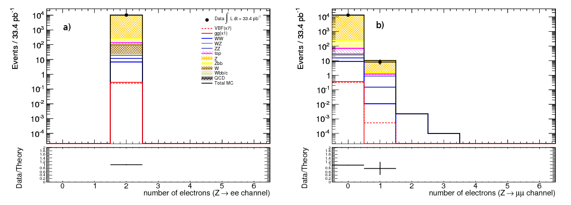
Because the leptons in the signal are from a decaying Z, they are of the same flavour and have opposite electric charge. However, inefficiency in the measurement of electrons means that approximately 5 $ \% $ of signal events with two electrons do not have opposite charge. This is represented in Figure 25, in which distributions of the product of selected lepton charges in a) the $ \ztoee $ and b) the $ \ztomm $ channels respectively are shown. If the leptons are of opposite charge, the product of their charges is -1, otherwise it is +1. The mis-measurement of electron charge is seen in the signal by the overflow into the +1 bin. In order to retain as much signal as possible, only in the muon channel is the requirement of opposite sign leptons made. To summarise the lepton selection requires exactly two electrons or muons satisfying the respective lepton selection. Selected muons are required to have opposite electric charge. All plots presented in the remainder of this section have been made requiring this lepton selection.

After applying the lepton selection just detailed, an already very large suppression of QCD backgrounds is achieved, with its efficiency reduced to 2 $ \times $ 10 $ ^{-9} $. In the same way the W+jets background is strongly suppressed, now with an efficiency of 1 $ \times $ 10 $ ^{-4} $. By far the dominant background at this stage is Z+jets due to its very large cross section and high survival rate of the lepton selection. It makes up over 90 $ \% $ of the total background. It is interesting to note that the $ \ztott $ +jets contribution is almost negligible compared to the contribution from $ \ztommee $ +jets. The efficiency of the GF and VBF components of the signal show similar performance at this stage of the selection, with approximately 35 $ \% $ of signal being retained ($ \mH $ = 200, 300 $ \Gcs $).

The performance of the selection appears to be similar in both the electron and muon channels, a trend which is apparent for all backgrounds with two leptons in the hard process. A different situation is seen for W+jets and QCD samples and typically samples which are not expected to have two real leptons. It is possible this is due to higher fake rates for electrons when compared to muons. Overall, about 30 $ \% $ more background events are found in the muon channel as opposed to the electron channel. Fairly good agreement is seen between data and Monte Carlo. Worse agreement is seen in the electron channel. It is plausible this may be due to the use of crack electrons which were shown to be less well modelled in the Monte Carlo.

Figure 25: Distribution of products of lepton charges for a) $ \ztoee $ and b) $ \ztomm $ channels for the $ \mH $ = 200 $ \Gcs $ sample and backgrounds (stacked).

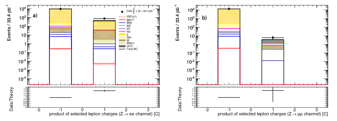
Di-lepton Invariant Mass

The decay of one of the Higgs Z's into leptons implies that if the two leptons are reconstructed their mass should be close to the nominal Z mass. This characteristic of the signal is exploited by requiring the reconstructed di-lepton mass ($ \mll $) to be within a window of the nominal Z mass. An initial cut of $ |\mll-\mZ| < $ 20 $ \Gcs $ is used, where $ \mZ $ = 91.1876 $ \Gcs $ is the nominal Z mass [4]. A slight deficit is seen when data and Monte Carlo are compared. This is largely an effect from the electron channel and is thought to be due to the use of crack electrons.

This cut is particularly efficient at rejecting backgrounds without decaying Z's and as such the backgrounds WW and W+jets are both reduced by approximately 70 $ \% $. Backgrounds with a top quark decay are also reduced by a similar factor. QCD is further suppressed by approximately 80 $ \% $. As expected the di-lepton mass window cut does not serve further to reduce backgrounds containing a real Z and as such Z+jets remains by far the largest background still making up over 90 $ \% $ of the total background. Good agreement of data and non-pile-up Monte Carlo was found.

Missing Transverse Energy ($ \etmiss $)

The presence of two neutrinos from the decay of one of the Z bosons in the signal topology means that a significant amount of missing energy is present. In contrast backgrounds without any neutrinos in the final state should not have any associated missing energy, apart from detector inefficiencies. Therefore a cut on missing energy should be very efficient at rejecting backgrounds such as $ \ztoll $ +jets and QCD. As the Higgs boson becomes more massive its decay products become more and more boosted, giving rise to more $ \etmiss $. This behaviour can be seen in Figure 26a) where the $ \etmiss $ in the signal samples as a function of Higgs mass is shown. In order to take advantage of this effect, at this stage in the analysis a low and high mass selection is proposed. The low mass selection is aimed at signal masses between $ \mH $ = 200 and 300 $ \Gcs $. In this region, $ \etmiss $ does not provide much discrimination between signal and background. A comparison between data and Monte Carlo for the $ \etmiss $ distribution is shown in Figure 26b). A clear discrepancy between data and Monte Carlo is seen for $ \etmiss < $ 40 $ \GeV $, where the Monte Carlo is seen to underestimate the data. This is shown in Figure 26c) to be a result of pile-up, in which a much improved agreement to the data is seen by using the pile-up reweighted Monte Carlo. This disagreement is understood as the low $ \pt $ jets from pile-up in the data contributing to higher levels of low $ \etmiss $ events. To avoid using this regime, for the low mass selection a baseline $ \etmiss > $ 40 $ \GeV $ cut is applied. The high mass selection is aimed at $ \mH \geq $ 300 $ \Gcs $, where the signal has enough $ \etmiss $ to provide substantial discrimination against background. For the high mass selection a baseline cut of $ \etmiss > $ 55 $ \GeV $ is used.

As expected due to their intrinsic lack of missing energy, the missing energy cut strongly suppresses Z+jets background and further suppresses QCD, which are both reduced by over 90 $ \% $ in the low mass selection. At this stage in the analysis, while Z+jets remains the largest background, the contribution from top becomes significant compared to Z+jets, having only been reduced by a comparable 25 $ \% $ with the low mass selection $ \etmiss $ cut. It is interesting to note that the contribution of single top is only a few percent of the total top background. It is strongly suppressed with the lepton selection and the di-lepton mass cuts because of the lack of two real leptons (especially in t channel production which makes up a large fraction of the single top contribution).

The $ \etmiss $ cut in the low mass selection also reduces the signal by up to 40 $ \% $ in the case of the $ \mH $ = 200 $ \Gcs $ sample. However, this is by far outweighed by the very large suppression of the total background, giving rise to an improvement in signal significance (defined as $ s/\sqrt{b} $ , where $ s $ is signal and $ b $ is total background normalised to luminosity analysed in the data) relative to that after the di-lepton mass window cut of approximately a factor of 10, which is largely attributed to the strong suppression of the Z+jets background.

Figure 26: Distribution of $ \etmiss $ for a) $ \mH $ = 200-600 $ \Gcs $ signal samples in 100 $ \Gcs $ steps, b) the $ \mH $ = 200 $ \Gcs $ sample and backgrounds (stacked). The effect of pile-up on the distribution is shown in c) for the total background.

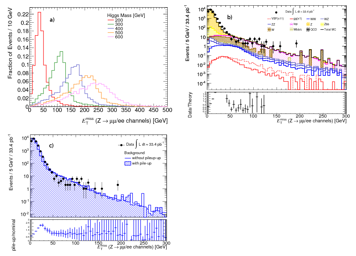
Leptons $ \Delta\phi $

A further consequence of the Higgs decay products becoming more boosted with increasing Higgs mass is that the difference in $ \phi $ between the leptons coming from the Z decay is reduced. This trend is shown in Figure 27 a), which shows the $ \Delta\phi $ between the identified leptons as a function of Higgs mass. Figure 27 b) shows agreement between data and Monte Carlo for this variable is fairly good and the effect of pile-up on the total background is negligible. The same was found to be true for signal. For the low mass selection $ \Delta\phi > $ 0.5 is required and in the high mass selection $ \Delta\phi < $ 2.0 is used.

Figure 27: Distribution of $ \Delta\phi $ between selected reconstructed leptons for a) each signal sample with $ \mH $ = 200-600 $ \Gcs $ in steps of 100 $ \Gcs $ and b) all backgrounds stacked with data and $ \mH $ = 200 $ \Gcs $ signal sample overlaid.

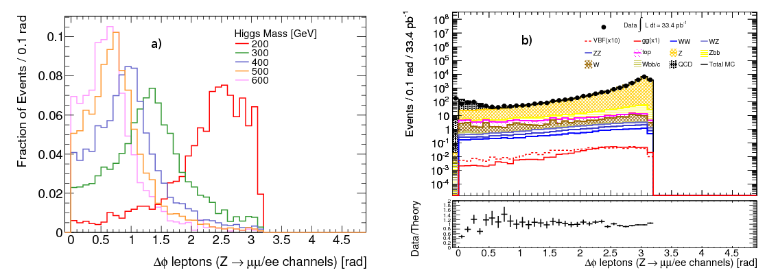
The $ \Delta\phi $ cut appears to have similar impact on most of the backgrounds in the low mass selection, decreasing total background by approximately 10 $ \% $, while there is little expected change in the signal level. The effect of the cut is more prominent in the high mass selection, decreasing total background by 50 $ \% $. The most affected backgrounds are those with a Z, reduced by approximately 50 $ \% $ each. In the high mass selection the main background now becomes $ \toptop $, which makes up 40 $ \% $ of the total background. In the low mass selection Z+jets remains the dominant background. A larger discrepancy between data and Monte Carlo is seen for the high mass selection. This is thought to be due to the low $ \Delta\phi $ region, perhaps due to poorly understood QCD normalisation.

b-jet veto

B-tagging (identification of hadronising b quarks) should provide efficient rejection of backgrounds with b hadron decays. Events are rejected if they have any jet identified using the jet selection criteria detailed with $ \pt > $ 25 $ \Gcs $ and $ |\eta| < $ 2.5 and with a SV0 b-tagging weight > 5.72. A plot of the highest SV0 b-tagging weight of all jets satisfying the standard jet selection, for events passing the lepton selection, clearly shows that the largest contribution of background satisfying the b-jet veto requirement comes from top quark backgrounds. This was further verified by a comparison of the efficiency of the b-jet veto as a function of the jet $ \pt $, made for the $ \mH $ = 200 $ \Gcs $ signal and the $ \toptop $ background. In the signal an efficiency above 90 $ \% $ is maintained across the entire $ \pt $ range whereas in the $ \toptop $ sample the efficiency reduces with jet $ \pt $ from around 50-60 $ \% $ for jet 50 < $ \pt $ < 100 $ \Gc $. A fluctuation in efficiency appears for jet $ \pt > $ 200 $ \Gc $ in the $ \toptop $ sample due to the low statistics of higher $ \pt $ jets passing the b-jet veto. Fairly good agreement between Data and Monte Carlo was seen. In particular the effect of pile-up on the SV0 jet weight distribution for the signal and total background was investigated and in both cases the effect found to be small.

The cut on SV0 tagging weight is negligible on all backgrounds other than those with b hadron decays, either from the decay of a top quark or b quarks in production with Z or W. These samples are suppressed by a further 30 $ \% $ or more. An increase in significance of just less than 10 $ \% $ is achieved in the low mass selection, similar to that seen in the high mass selection.

Transverse Mass ($ \mT $)

As there are two neutrinos in the signal final state the Higgs mass cannot be fully reconstructed. An approximation to this is to use the transverse mass $ \mT $. The definition of transverse mass used in this analysis is $$ \begin{equation} m_{\mathrm{T}} = {\Big(\sqrt{\mathrm{m_{Z}}^{2} + |\vec{p_{\mathrm{T}}}(ll)|^{2}} + \sqrt{\mathrm{m_{Z}}^{2} + |\vec{p}_{\mathrm{T}}^{\mathrm{miss}}|^{2}}\Big)}^{2} - (\vec{p_{\mathrm{T}}}(ll) + \vec{p}_{\mathrm{T}}^{\mathrm{miss}})^{2} \label{eqn_mt} \end{equation} $$

where $ \mathrm{m_{Z}} $ is the nominal Z mass, $ \vec{p_{\mathrm{T}}}(ll) $ refers to the $ \pt $ vector of the leptons and $ \vec{p} $ the missing transverse momentum. Figure 28a) shows how for the signal the peak of the $ \mT $ distribution falls approximately on the corresponding Higgs mass. From Figure 28b) the background distribution has a shape similar to the 200 $ \Gcs $ signal and as such this is where discrimination is worst. As such no cut is placed on $ \mT $ in the low mass selection. With increasing Higgs mass better discrimination is achieved as more $ \etmiss $ is present in the signal. For the high mass selection a baseline cut of $ \mT > $ 200 $ \Gcs $ is applied.

Figure 28: Distribution of $ \mT $ for a) $ \mH $ = 200-600 $ \Gcs $ signal samples in 100 $ \Gcs $ steps and b) the $ \mH $ = 200 $ \Gcs $ sample and backgrounds (stacked).

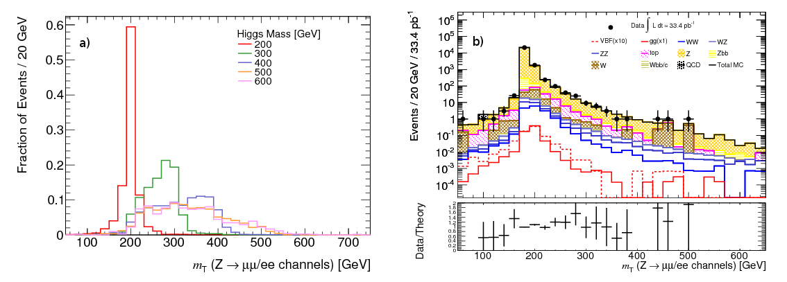
Selection of remnants of VBF process

In the following the set of cuts used to exploit the VBF topology in the signal is discussed. This will be referred to as the tag-jet selection whereby tag-jets is used to refer to the jets identified as originating from the VBF process. The tag-jet selection begins by requiring at least two jets passing the jet selection ($ \mathrm{N}_{\mathrm{jets}} \geq $ 2), because as cross checked signal events produced via VBF will typically have two reconstructed tag-jets. Clearly the requirement of two jets passing the jet selection provides very good rejection of backgrounds like Z+jets. The jets associated with the VBF remnants are assumed to be the two highest $ \pt $ jets in the event, which is one of the most common ways to identify them [40].

Effect of overlap removal on tag-jets

As discussed in the section Overlap Removal, within this analysis jets overlapping geometrically with electrons or muons passing the quality requirements are removed from consideration. By far the dominant type of overlap is between electrons and jets. In the following study where the $ \mH $ = 200 $ \Gcs $ signal sample was used, the total fraction of electron-jet overlaps out of all the overlaps was found to be over 99 $ \% $. It is important that the overlap removal does not remove the identified tag-jets. In the study performed the identified reconstructed tag-jets were matched to the truth quarks associated with the VBF topology (VBF quarks) using $ \Delta R $ matching. The $ \Delta R $ between each possibility of truth-reconstructed quark-tag-jet was calculated and the smallest summed total value then taken to establish which reconstructed jet is compared to which truth VBF quark. This was done separately for the $ \ztoee $ and $ \ztomm $ channels. The same procedure was then performed using the reconstructed jets removed in the overlap removal procedure, to find those which most closely matched the truth VBF quarks. Figure 29a) shows a comparison of the difference in $ \pt $ between each identified reconstructed tag-jet ( $ \pt $ (reco)) and the corresponding matched truth VBF quark ( $ \pt $ (truth)) as a function of the truth VBF quark $ \pt $. It shows that in both the electron and muon channels there are reconstructed jets left after the overlap removal that far more accurately mimic the VBF quarks than those which are removed in the overlap removal process. This behaviour is seen across most of the $ \pt $ range investigated, indicating it is rare that the overlap removal process is rejecting jets which are very likely to be the identified tag-jets.

The same behaviour is less apparent as a function of truth VBF quark $ \eta $ shown in Figure 29b). However, this behaviour is further backed up in Figures 29c) and 29d), where it is shown there is a much improved agreement in terms the minimum $ \Delta R $, $ \Delta R_{\mathrm{min}} $, between truth VBF quarks and the best matched jets not removed by the overlap procedure compared to those removed (Figure 29c)) and this is verified if a comparison is made of the $ \eta $ distribution of the jets removed by the overlap removal and the truth VBF quarks (Figure 29d)).

Figure 29: $ \pt $ (truth)- $ \pt $ (reco)/ $ \pt $ (truth) plotted as a function of truth VBF quark (a) $ \pt $ and (b) $ |\eta| $ for the reconstructed jets best matched to the truth VBF quarks and the jets removed by the overlap removal procedure. (c) shows the $ \Delta R $ between truth VBF quarks and best matched/overlap removed reconstructed jets and (d) the $ \eta $ of truth VBF quarks and overlap removed tag-jets (the asymmetry of this distribution for the overlap removed tag-jets is caused by the OTX cut in the electron selection). Signal corresponds to the $ \mH $ = 200 $ \Gcs $ Higgs sample.

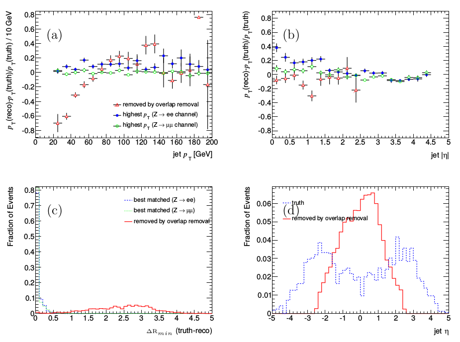
Tag-jet Kinematics

The tag-jets in the signal are derived from the hard process and result from recoiling against the Higgs boson. Because of this they tend to be harder than the jets found in the backgrounds. This behaviour is shown in Figure 30a) where the $ \pt $ of the leading tag-jet is shown. It is plotted requiring the lepton selection detailed previously as well as two or more jets passing the quality requirements detailed. This is true of all subsequent plots shown in this section. The leading tag-jet $ \pt $ appears to provide good discrimination over backgrounds and a baseline cut of > 40 $ \Gc $ is implemented.

As discussed in the section Signal Processes a characteristic feature of VBF is that the tag-jets tend to be in the forward regions of the detector and well separated in pseudo-rapidity. Therefore the tag-jets are required to be in opposite hemispheres of the detector (i.e. the product of the $ \eta $ of the two tag-jets ($ \eta\times\eta $ (tag-jets)) must be negative). In addition, a cut on the $ \Delta\eta $ between the tag-jets is made and required to be greater than 3.0. The result of the large pseudo-rapidity separation between tag-jets is that the invariant mass of the tag-jets tends to be large compared to all backgrounds. The invariant mass of the two tag-jets is required to be greater than 400 $ \Gcs $ in the low mass selection. These properties are illustrated in Figure 30. Due to the large background suppression provided by the larger possible $ \etmiss $ cut, no cut on the mass of the tag-jets is made in the high mass selection.

Figure 30: Distributions related to the kinematics of the tag-jets, a) $ \pt $ of leading tag-jet, b) $ \eta $ x $ \eta $ of tag-jets, c) $ \Delta\eta $ between tag-jets and d) mass of tag-jets. Each background contribution is shown stacked. VBF and GF components for the $ \mH $ = 200 $ \Gcs $ are included.

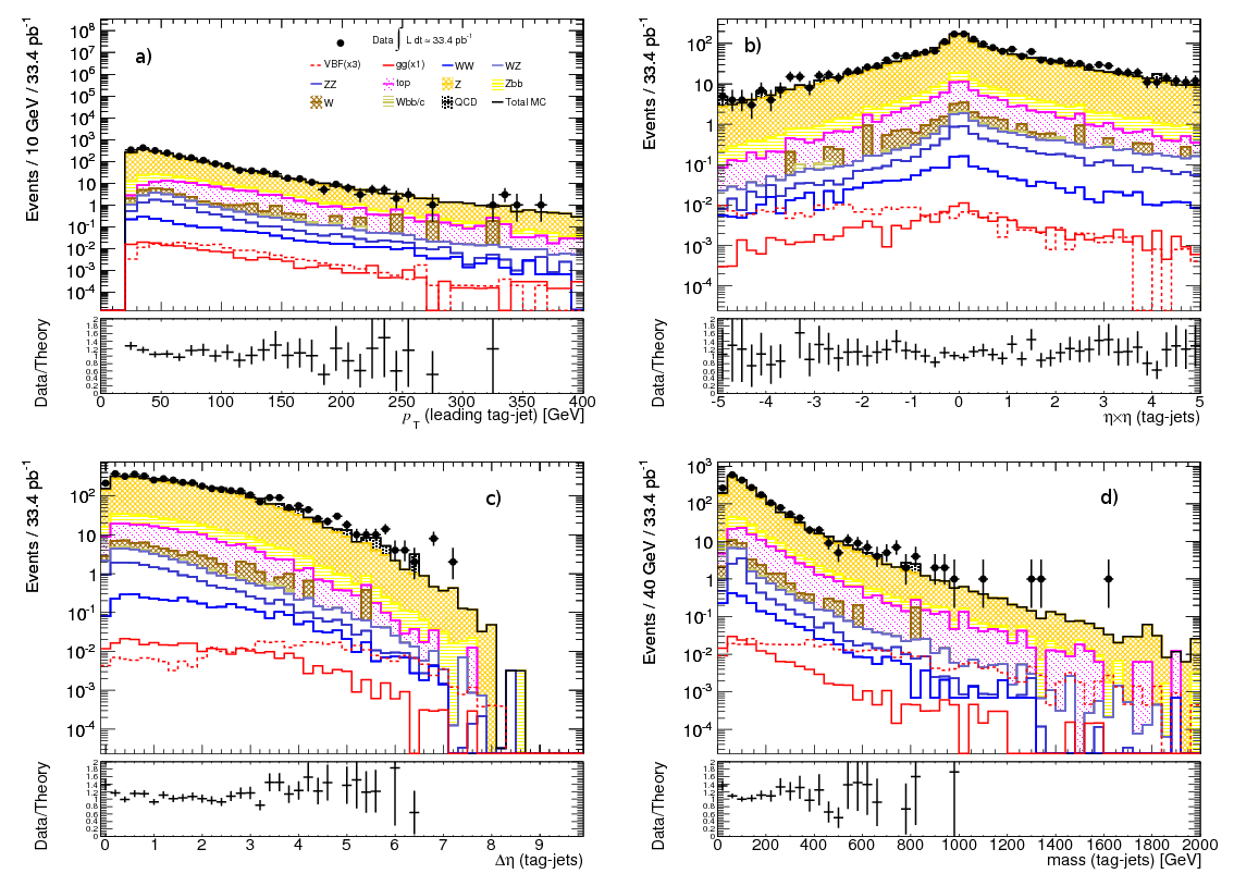
Central Jet Veto

The absence of colour exchange between the partons within the VBF process means that jet activity in the signal in the central region is suppressed. Therefore it is beneficial to reject (veto) events with additional jets (referred to here as non tag-jets). This cut is commonly called a central jet veto (CJV). In the low mass selection a CJV cut is adopted, removing events with non tag-jets with $ \pt > $ 20 $ \Gc $ and $ |\eta| < $ 3.2.

Effect of cuts

After requiring at least two jets passing the jet selection, the GF component of the signal is reduced by 70 $ \% $ for the $ \mH $ = 200 $ \Gcs $ signal when compared to the yield at the end of the selection relating to the Higgs decay products while the VBF component is reduced by 25 $ \% $. The backgrounds suppressed the most correspond to those without hard jets, namely the di-boson backgrounds which reduce by as much as 90 $ \% $. However, the main background Z+jets is further reduced by over 50 $ \% $ in the low mass selection. This reduction is less pronounced for the high mass selection. It is thought this is because of the larger $ \etmiss $ cut only allowing Z events with large jet activity to survive. W+jets background which was the second largest background at the end of the selection relating to the Higgs decay products in both the low and high mass selections is now reduced by over 80 $ \% $ in each case by applying this cut, becoming a minor background. Top background from $ \toptop $ does not experience a major drop in efficiency and together with Z+jets forms over 80 $ \% $ of the total background in both the low and high mass selections. At this stage in the selection data and Monte Carlo are not in agreement, data having approximately double the number of events than found in the Monte Carlo. Comparing the multiplicity of jets satisfying the jet selection for the nominal Monte Carlo and the pile-up reweighted Monte Carlo, shows the pile-up Monte Carlo predicts a larger contribution than the nominal Monte Carlo for jet multiplicities between one and three, verifying that the discrepancy observed between data and Monte Carlo after this cut is due to pile-up.

The leading tag-jet $ \pt $ cut in both the low and high mass selections is most effective at reducing W+jets background, which is reduced by approximately 50 $ \% $. All other backgrounds are affected similarly and reduce by around 10 $ \% $ or less. Z+jets and top remain the main backgrounds constituting around 50 and 25 $ \% $ of the total background respectively in both the low and high mass selections.

Despite reducing signal efficiency by around 1/3 in the low mass selection (there is negligible loss in the high mass selection), the total background is reduced by over twice this amount by the requirement that the tag-jets lie in opposite hemispheres. This gives an increase in significance of around 20 $ \% $ in both the low and high mass selections. It is interesting to note that data and nominal Monte Carlo now agree again within statistical error. It is thought this occurs because in the current selections, the events selected by the leading tag-jet and opposite hemispheres requirement tend to select events where there is agreement between data and Monte Carlo in terms of the jet multiplicities, corresponding to events with four or more jets.

The $ \Delta\eta $ cut provides a further large reduction in total background, by as much as 80 $ \% $ in both selections. This is largely due to the strong suppression of what still remains the largest background, Z+jets. The signal is largely unaffected in each selection, resulting in an increase in signal significance by over 50 $ \% $ in each case. At this stage in the selection, just one data event remains in the low mass selection while no events survive the high mass selection. It is thought the discrepancy between data and Monte Carlo is still largely due to pile-up effects. This was verified by comparing the tag-jet variable distributions for non pile-up and pile-up reweighted Monte Carlo. In particular, the variables N $ _{\mathrm{jets}} $ and $ \Delta\eta $ are shown not to agree, with the non pile-up Monte Carlo underestimating the pile-up Monte Carlo. However, for the other variables considered pile-up and non pile-up Monte Carlo are observed to agree within error.

As expected the CJV has little effect other than on those backgrounds expected to have a non-negligible amount of jet activity, namely $ \toptop $ and Z+jets background. The largest decrease is seen for $ \toptop $ at approximately 50 $ \% $. A negligible increase in signal significance is observed.

The cut on the mass of the tag-jets removes the remaining W statistics and leads to a reduction of the Z+jets and $ \toptop $ backgrounds by 60 $ \% $ or more in each selection contributing to a increase in signal significance by around 40 $ \% $.

Results of Baseline Selection

In this section a baseline analysis was presented for the cut-based selection of the VBF $ \htollnunu $ signal. The selection is summarised in the following. Where there is a difference between low and high mass selections this is indicated with the low mass cut value defined and next to it the high mass cut value in brackets.

Lepton Selection: Two electrons or muons passing requirements outlined. No other leptons of any other type. Opposite sign requirement made in muon channel.
Di-lepton mass window: $ |\mll-\mZ| $ < 20 $ \Gcs $.
$ \etmiss $ : > 40(55) $ \GeV $ .
$ \Delta\phi $ : Between leptons > 0.5(<2.0) rad.
b-jet veto: Reject any event with a jet with SV0 weight > 5.72.
$ \mT $ : no cut(> 200) $ \Gcs $.
$ \mathrm{N}_{\mathrm{jets}} \geq $ 2: At least two jets passing the standard selection.
leading tag-jet $ \pt $: > 40 $ \Gc $
$ \eta\times\eta $: Product of tag-jets absolute $ \eta $ must be less than 0, i.e. tag-jets must be in opposite hemispheres.
$ \Delta\eta $: > 3.0(no cut).
CJV: Reject events with non tag-jets with $ \pt > $ 20 $ \Gc $ and $ |\eta| < $ 2.5 (no cut).
mass tag-jets: > 400(no cut) $ \Gcs $.

A number of samples have zero Monte Carlo events after the selection detailed, including QCD, W+jets, single top and Z $ \rightarrow \tau\tau $ +jets. Other samples have zero Monte Carlo events surviving for particular physical processes. The effect on the final expected background rate when the zero surviving Monte Carlo events in these samples is replaced by one was checked. Although this method will overestimate the background, as in all cases the final efficiency of each sample is less than the inverse of the total number of initial Monte Carlo events, it does provide a crude means by which background contributions which might otherwise be neglected can be approximated. It was seen that the increase in background rate observed was within statistical error. However, for samples where no Monte Carlo events remain after the selection, potentially large increases in background rate are predicted using this method, particularly for QCD and W. Therefore an attempt is made to try and estimate their effect in the following section.

Estimation of QCD, W, Z $ \rightarrow\tau\tau $ +jets and single top contributions

It has been shown that the contributions from the QCD, W, $ \ztott $ +jets and single top backgrounds could not be estimated very reliably due to lack of Monte Carlo statistics. Here we use an alternative approach to estimate these background contributions.

The approach used to estimate their contribution, called factorization, relies on the property that if a set of cuts A are independent to those in set B, then the efficiency after applying cuts A and B together is the same as multiplying the efficiency found by applying cuts A independently of set B by the efficiency of applying cuts B independently of cuts A as shown in Eqn. \eqref{eqn_CutFactorization}. $$ \begin{equation} {\epsilon}_{AB} = \epsilon_{A} \times {\epsilon}_{B} \label{eqn_CutFactorization} \end{equation} $$

In general, this holds for any number of sets of cuts provided each set is independent of the other. In the following three different sets of cuts are identified as independent in the analysis, those relating to the lepton cuts, the $ \etmiss $ cut and the tag-jet cuts

Lepton cuts: relaxed lepton selection and di-lepton mass window.
$ \etmiss $ cut: $ \etmiss > $ 40 $ \GeV $.
tag-jet cuts: N $ _{\mathrm{jets}} \geq $ 2, each with $ \pt $ > 20 $ \Gc $ , $ |\eta| $ < 4.5. Highest $ \pt $ jets $ \eta\times\eta $ and $ \Delta\eta $ as in baseline selection.

The relaxed lepton selection requires either two medium electrons or two combined or segment tagged muons (one of which must be combined). In the electron channel the electron cluster must have $ \et > $ 20 $ \GeV $ and the electron track $ |\eta| < $ 2.5. In the muon channel, the muon is required to have $ \pt > $ 20 $ \Gc $ and $ |\eta| < $ 2.5. This more relaxed set of cuts is used to maximise the acceptance of the samples considered (particularly QCD) and means that the estimated contributions are expected to be less than the values determined.

The efficiencies of applying each individual set of cuts on each sub-sample making up the QCD, W+jets, $ \ztott $ +jets and single top backgrounds are computed. All the available statistics have been used in each case. The contribution to the total background of each sub-sample is then estimated by finding the product of efficiencies from applying each set of cuts and using this to find the expected number of events for each sub-sample. Overall the contribution from QCD is expected to be less than 3.1 $ \times $ 10 $ ^{-2} $ events and that from W less than 3.5 $ \times $ 10 $ ^{-2} $ events. The contribution from $ \ztott $ +jets and single top is much less at 7.6 $ \times $ 10 $ ^{-4} $ and 2.0 $ \times $ 10 $ ^{-3} $ respectively, making the total contribution of these samples within the statistical error on the total background.

Optimization of Feature Selection cuts

In this section the baseline cut-based selection outlined in the section Feature Selection is optimized. This is done in a two step procedure in which first the variables relating to the tag-jet selection are optimized and then variables relating to the Higgs decay products are optimized. The effect of different methods to tag the jets from the VBF remnant and different measures of the overall performance of the optimization are compared. Each optimization step is carried out at each available mass signal sample. A comparison between the baseline and optimized selection is made.

Optimization procedure

In order to establish an optimized event selection the procedure adopted was to compare different cut configurations and rank them according to a figure of merit, or significance measure by which the signal to background ratio is optimal given the inputs to the optimization. Several different definitions are typically used to define the signal significance for an analysis. The most widely used definitions are shown in Eqns. \eqref{zone} and \eqref{ztwo}. $ \mathrm{Z_{1}} $ is valid in the Gaussian limit when signal ($ s $) and background ($ b $) are much greater than unity. In the Poisson limit, this definition is approximate and only valid when $ s $ << $ b $ and $ s $ and $ b $ are known to a high accuracy. In this analysis it has been shown that $ s $ << $ b $ and therefore it is expected that this definition is suitable. However, $ \mathrm{Z_{2}} $ [41] is a more general definition of $ \mathrm{Z_{1}} $ in that it is valid when $ s $ >> $ b $ in the Poisson limit. In the following both measures are compared. $$ \begin{equation} \mathrm{Z_{1}} = \frac{s}{\sqrt{b}} \hspace{1cm} \label{zone} \end{equation} $$ $$ \begin{equation} \mathrm{Z_{2}} = \sqrt{2((s+b)ln(1+\frac{s}{b})-s)} \label{ztwo} \end{equation} $$ The optimization procedure takes into account correlations between the cuts being optimized by considering each possible combination of cuts, i.e. performing an optimization in an $ n $ dimensional cut-space, where $ n $ is the number of different cut variables being optimized. Due to the large CPU time required to perform optimization done in this way (number of combinations = Number of Cuts per Variable $ ^{n} $ ) a method other than considering each combination of cuts was developed and was used to derive results shown in this section. In this method, the cut combinations are ordered in increasing tightness and information of what the previous cut combination passed is used to identify which subsequent cut should be considered. Through this method, intermediate combinations are assigned as being passed or failed depending on whether the cuts are looser or tighter and this allows for the computation time of evaluating the total cut-space to be drastically reduced. Results using this method were compared to the more time consuming method of considering each combination in turn for a variety of different situations, where the number of variables and the number of cuts per variable was made different. Agreement between the two methods was found in all cases.

The identification of an optimal set of cuts using the optimization procedure outlined is done using an independent Monte Carlo (training) sample with the same size as that used to produce the results of the baseline selection (testing sample). Final results using the optimized cuts will be quoted using the testing sample so that a direct comparison of each selection can be made. All processes are used in the optimization apart from those contributing to QCD and W+jets because the available statistics is too small. However, as shown in the section Estimation of QCD, W, Z $ \rightarrow\tau\tau $ +jets and single top contributions these background are expected to have negligible contribution to the overall background after all cuts are applied.

Optimization of tag-jet selection

The variables considered in the optimization of variables related to the VBF remnants included the leading tag-jet $ \pt $, the requirement that the tag-jets be in opposite hemispheres ($ \eta\times\eta $), the $ \Delta\eta $ between the tag-jets, the mass of the tag-jets and the $ \pt $ of non tag-jets within $ |\eta| < $ 3.2. The ranges and step sizes considered for each of the variables considered is shown below. In each case the possibility of applying no-cut was also tested.

leading tag-jet $ \pt $ > 20-65 $ \Gc $ in steps of 5 $ \Gc $.
$ \eta\times\eta $ < 0.
$ \Delta\eta $ > 3.2-4.8 in steps of 0.2.
$ \pt $ (non-tag-jets) 5-95 $ \Gc $ in steps of 10 $ \Gc $.
mass (tag-jets) 300-750 $ \Gcs $ in steps of 50 $ \Gcs $.

In order to ensure that the background events used in the optimization process are relevant to the search in the VBF $ \htollnunu $ channel, events are required to pass the lepton selection, $ \etmiss $ and Z mass selections from the baseline selection. Attempts were made to perform the optimization loosening these cuts further to maximise statistics available. Typically however, these optimizations tended to select very hard optimal cuts far outside what would generally be used in a VBF analysis. This is because of the overwhelming Z+jets background which has to be dealt with, in particular, once $ \etmiss $ is loosened to below 30 $ \GeV $. Because of these problems the low mass selection baseline cuts relating to the Higgs decay products were adopted in the optimizations performed of the VBF related variables and used to produce the results shown subsequently. However, requiring this selection meant that there were very limited statistics with which to perform the optimization. In an attempt to avoid problems associated with allowing the optimization to explore regions of cut space that are not well understood due to lack of statistics, for each combination of cuts, when a certain sample runs out of Monte Carlo statistics, then the contribution from this background is estimated by assuming one surviving Monte Carlo event. The total background found using this method is then required to be less than the sum of the total background calculated without this replacement and its associated error, in order for the combination of cuts to be considered as valid. Distributions showing the maximum significance as a function of cut value were produced and showed no large difference between each significance measure. The most discrimiminating variable was found to be the $ \Delta\eta $ cut. The optimization was repeated for each Higgs mass considered. Using the inputs described, the optimal cut positions are fairly independent of Higgs mass. Each significance measure is shown to select the same optimal cut positions.

Comparison of methods to tag the jets from the remnants of the VBF process

As discussed in the section The Higgs Mechanism the tag-jets in VBF analyses are most commonly identified using the two highest $ \pt $ jets. In the following a comparison is made between this approach and two other methods: i) considering the tag-jets as the two jets with the highest invariant mass and ii) the two jets with the largest separation in $ \eta $. The best performing method is then subsequently compared to the more conventional one of using the highest $ \pt $ jets by re-performing the optimizations of the previous section.

In order to make a comparison of these different methods, the minimum combined $ \Delta R $ between the tag-jets identified with each method and the quarks generating the VBF topology (subsequently referred to as truth VBF quark's, required to have $ \pt > $ 20 $ \Gc $ and $ |\eta| < $ 4.5) was found. This study was done using the $ \mH $ = 200 $ \Gcs $ signal sample. Reconstructed jets satisfying the criteria to be used in the analysis were used. The same was done for the best matched pair of reconstructed jets. In order to establish a matching efficiency, the $ \Delta R $ between each truth VBF quark and its matched reconstructed jet was required to be less than 0.2. Using this definition the best matched reconstructed jets are found to satisfy this criteria for approximately 70 $ \% $ of events in truth $ \ztoee $ events and around 75 $ \% $ of events in truth $ \ztomm $ events for the $ \mH $ = 200 $ \Gcs $ signal sample. Selecting tag-jets based on the highest $ \pt $ and mass jets was shown to give a similar performance in truth $ \ztomm $ events, whereby an efficiency of around 90 $ \% $ with respect to the best matched scenario is achieved in each method. However, in truth $ \ztoee $ events the performance of selecting tag-jets based on highest mass gives an improvement of over 10 $ \% $ compared to using the highest $ \pt $ jets. This trend was also indicated by comparing the $ \pt $ difference between reconstructed and truth VBF quarks as a function of truth VBF quark $ \pt $ and $ |\eta| $ for truth $ \ztommee $ events in the $ \mH $ = 200 $ \Gcs $ signal sample. The performance of using the jets with the largest separation in $ \eta $ also shows an improvement over the method using highest $ \pt $ jets in truth $ \ztoee $ events but is worse in truth $ \ztomm $ events. However, its performance is worse compared to the method using the highest mass tag-jets and so is not discussed further.

In order to try and better establish if selecting tag-jets based on highest mass jets in the event provides an improvement over using the highest $ \pt $ jets, the two methods were compared by re-running the optimization procedure as detailed earlier in this section using the tag-jets identified in the different methods. This is expected to provide a much more robust comparison of methods to tag the jets because it takes into account the signal and the background and chooses the method based on which provides better signal over background discrimination. The significance measure Z $ \mathrm{_{1}} $ was used. Each method appears to perform similarly, although the method using the highest $ \pt $ jets as the tag-jets yields a slightly higher significance. A similar trend was observed for the other signal mass points considered, and as such the method using highest $ \pt $ jets is adopted to obtain the optimized results.

Considering the little mass dependence of the optimizations performed, a fixed set of cuts relating to the VBF topology was applied across the mass points considered. The value of the cuts used was found by taking the average of the cut values found as a function of Higgs mass. The optimal cut values are leading tag-jet $ \pt > $ 25 $ \Gc $, requiring the tag-jets are in opposite hemispheres, $ \Delta\eta > $ 3.6, non tag-jet $ \pt > $ 45 $ \Gc $ and mass tag-jets > 450 $ \Gcs $.

Optimization of variables relating to Higgs decay products

The variables relating to the Higgs decay products were optimized using the same method as used to optimize the variables relating to the Higgs decay products. This was done using the Z $ \mathrm{_{1}} $ and Z $ \mathrm{_{2}} $ significance measures with cuts on the variables relating VBF topology fixed at the optimized values. The variables optimized, the cut range investigated and the step sizes used were

Lepton $ \pt $ >, 20-70 $ \Gc $ in steps of 5 $ \Gc $.
(di-lepton mass-$ \mZ $) <, mass 20-70 $ \Gcs $ in steps of 5 $ \Gcs $.
$ \etmiss $ >, 20-270 in steps of 25 $ \GeV $, then (selected-25)-(selected+25) $ \GeV $ in steps of 5 $ \GeV $.
$ \mt $ >, 0-500 in steps of 50 and then (selected-50)-(selected+50) in steps of 10 $ \Gcs $.

where in the case of $ \etmiss $, because of the large potential range of optimal cuts (taking into account varying Higgs mass), the optimization was done in two steps. First $ \etmiss $ in the range 20-270 $ \GeV $ in 25 $ \GeV $ steps was considered and then which ever cut was found to be the optimum (selected), the range (selected-25)-(selected+25) was then considered in steps of 5 $ \GeV $.

The optimal cuts for the low and high mass selections were obtained by averaging the optimal cuts found at each mass point in a similar way to when the optimization of the VBF related variables was done. For the low mass selection, the masses between $ \mH $ = 200-280 $ \Gcs $ were used and the optimal cuts identified as lepton $ \pt > $ 20 $ \Gc $, di-lepton mass window $ |\mll-\mZ| < $ 15 $ \Gcs $ and $ \etmiss > $ 40 $ \GeV $. For the high mass selection $ \mH \geq $ 300 $ \Gcs $ samples were used and the optimal cuts found to be lepton $ \pt > $ 20 $ \Gc $, di-lepton mass window $ |\mll-\mZ| < $ 15 $ \Gcs $ and $ \etmiss > $ 50 $ \GeV $.

Results of Optimization

In summary, the optimal cuts adopted for the low and high mass selections are

Lepton Selection: Two electrons or muons passing requirements outlined. No other leptons of any other type. Same flavour opposite sign requirement made in muon channel.
Di-lepton mass window: $ |\mll-\mZ| < $ 15 $ \Gcs $.
$ \etmiss $: > 40(50) $ \GeV $.
$ \Delta\phi $: Between leptons > 0.5(<2) rad.
b-jet veto: Reject any event with a jet with SV0 weight > 5.72.
$ \mT $: no cut(> 200) $ \Gcs $.
N $ _{\mathrm{jets}} $: $ \geq $ 2 jets passing selection outlined.
leading tag-jet $ \pt $: > 25 $ \Gc $
$ \eta\times\eta $: Product of tag-jets absolute $ \eta $ must be less than 0, i.e. tag-jets must be in opposite hemispheres.
$ \Delta\eta $: > 3.6(no cut).
CJV: Reject events with non tag-jets with $ \pt > $ 45 $ \Gc $ and $ |\eta| < $ 2.5 (no cut).
mass tag-jets: > 450 $ \Gcs $ (no cut).

Where there is a difference between the selections, the high mass selection is quoted in brackets. The method for estimating the contribution of W and QCD backgrounds discussed in the section Estimation of QCD, W, Z $ \rightarrow\tau\tau $ +jets and single top contributions applies to the optimal set of cuts because the cuts used to estimate their effect are tighter than those in the baseline. Applying the optimal cuts, the contribution of W and QCD backgrounds estimated using cut factorization is shown to be within the statistical error on the background. In the low mass selection for the $ \mH $ = 200 $ \Gcs $ signal, using the optimized selection an improvement in signal significance of just under 10 $ \% $ is observed. A similar effect is seen for the high mass selection for the $ \mH $ = 300 $ \Gcs $ signal. Signal efficiencies in both cases are maintained above 5 $ \% $.

Mass Dependance

A comparison between the baseline and optimized selections as a function of Higgs mass is shown in Figure 31. An improvement in significance (Z $ \mathrm{_{1}} $ ) of up to 10 $ \% $ is observed as a function of Higgs mass. Using the optimized cuts, the low mass selection performs markedly better than the high mass selection for Higgs masses up to $ \mH $ = 280 $ \Gcs $. Beyond this the high mass selection provides better discrimination over background. This is largely due to increasing $ \etmiss $ in higher Higgs mass signals. To maximise expected significance, one selection is adopted, with the low mass selection used for Higgs mass $ \mH $ < 300 $ \Gcs $ and the high mass selection for Higgs mass $ \mH \geq $ 300 $ \Gcs $. Adopting these selections, signal efficiency is maintained above 5 $ \% $ across all masses. However, it is seen to rise with increasing Higgs mass, to approximately 10 $ \% $ in the low mass selection for $ \mH $ = 280 $ \Gcs $ and to around 20 $ \% $ in the high mass selection for $ \mH $ = 600 $ \Gcs $. This is caused by the combination of increasing $ \etmiss $ in the signal with increasing Higgs mass and the fixed $ \etmiss $ cuts used. This is a favourable feature as the SM Higgs cross section decreases by over six orders of magnitude with increasing Higgs mass in the mass region considered. However, the change in cross section is the dominant effect, shown by the significance decreasing with increasing Higgs mass.

Figure 31: Comparison of results after applying baseline and optimized selections as a function of Higgs mass shown in terms of a) significance (Z=Z $ \mathrm{_{1}} $ ), b) expected number of signal (n $ \mathrm{_{s}} $ ) and background ( n $ \mathrm{_{b}} $ ) events for an integrated luminosity of 33.4 pb $ ^{-1} $ and c) signal ( $ \epsilon\mathrm{_{s}} $ ) and background ( $ \epsilon\mathrm{_{b}} $ ) efficiencies.

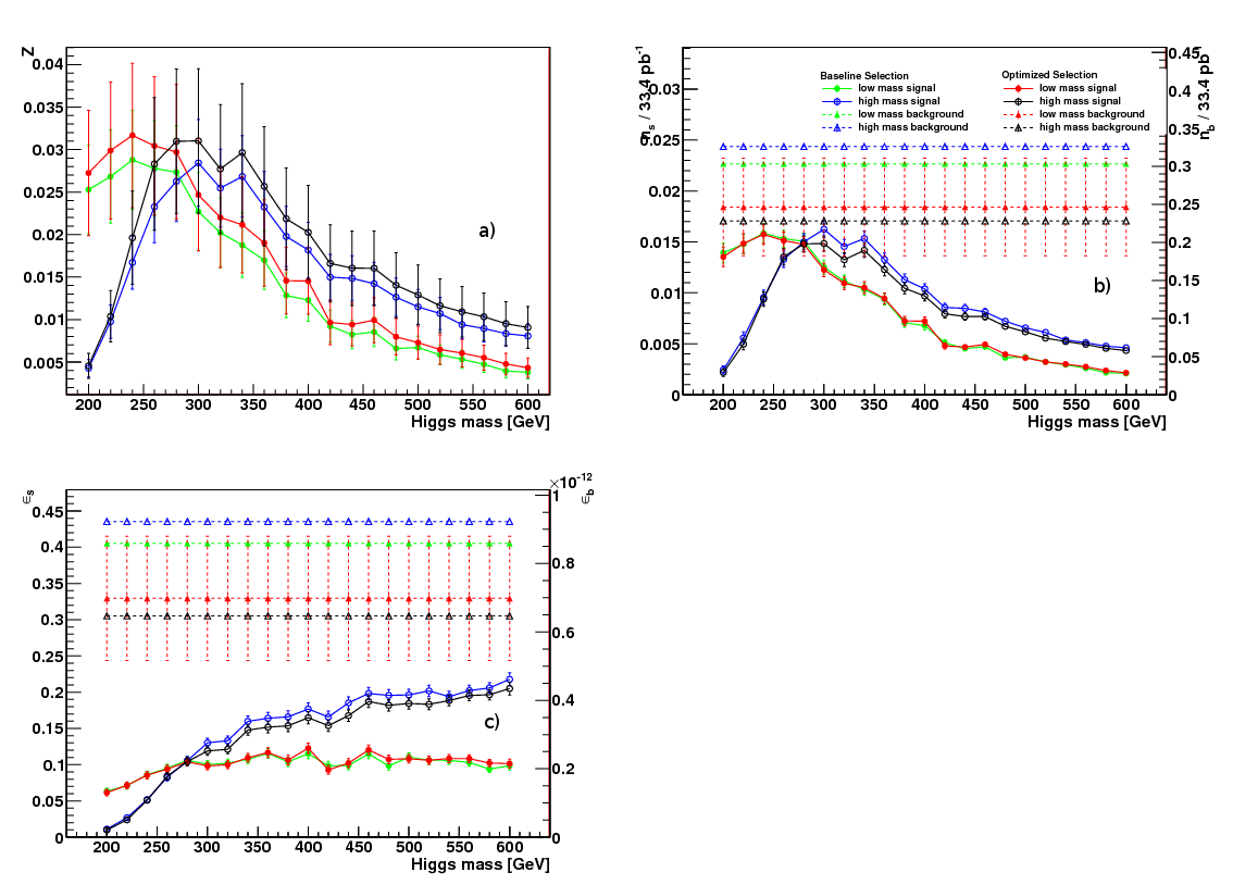
Systematic Uncertainties

This section explores a number of systematic effects which may lead to additional uncertainties on the search prescribed in the previous section. The systematic effects considered can be categorised into two types. The first type is those which give an uncertainty on the event yield and includes uncertainty on luminosity and uncertainty on signal and background cross sections. Methods to estimate the contribution of two of the main backgrounds, $ \toptop $ and Z+jets, are explored. The other type of uncertainty considered is that which results in an uncertainty on the acceptance efficiencies of the samples considered as a result of detector inefficiencies changing the kinematic distributions from which the analysis makes selections. In the studies presented these changes are explored in terms of their effect on the overall event yields. The combination of all systematic errors, added in quadrature, is used to define an overall systematic error in the rate of the total background and signal, for the low and high mass selections respectively. The section concludes with a discussion of the sensitivity of the search by way of 95 $ \% $ C.L. limits on the signal cross section relative to the SM prediction as a function of Higgs boson mass for the 2010 dataset.

Theoretical uncertainties

The cross sections for the processes used in this analysis have associated uncertainties due to imperfect knowledge of the parton distribution functions, the incomplete description of the parton showering process and modelling of the underlying event and dependence on renormalisation and factorisation scales. The uncertainty on the VBF process has been studied by the LHC Higgs cross section working group who estimate the uncertainty on the Standard Model Higgs boson cross section produced by VBF to be 3-9 $ \% $ [8] in the mass range considered in this analysis. A flat uncertainty of 6 $ \% $ is assumed in the following for each signal mass. The uncertainties on the background cross sections quoted in [20] are assumed. These uncertainties on the background cross sections, give rise to a total background uncertainty of $ \pm $ 8.5 $ \% $ and $ \pm $ 9.1 $ \% $ in the low and high mass selections respectively.

Data Driven Background Estimation

An important way in which the contribution from backgrounds in a search can be estimated, provided there is sufficient statistics, is by estimating them using data driven techniques. These techniques are merited as they allow reliance on predicted cross sections to be reduced and can also lead to reduced systematic uncertainties. Typically these methods rely on identifying control regions that are enriched with the backgrounds to be estimated by changing the selection cuts used in an analysis. An attempt was made to use these techniques to estimate two of the main backgrounds in this analysis, $ \toptop $ and Z+jets, by reversing the cuts in the optimized selection, to identify $ \toptop $ and Z+jets control regions.

Ideally one would like to be able to estimate the contribution of the main backgrounds in an analysis in the region of cut space defined by the selection, i.e. in the signal region. In order to estimate the contribution of a particular background in a signal region, a common approach is the ABCD method. In this method, the contribution of a background is estimated in the signal region A, by defining control regions (B and C) enriched with this background. A further control region, D, corresponds to the control region after applying B and C selections. The number of background events in the signal region, N $ _{\mathrm{A}} $ is then $$ \begin{equation} \mathrm{N}_{\mathrm{A}} = \frac{\mathrm{N}_{\mathrm{B}}}{\mathrm{N}_{\mathrm{D}}} \times \mathrm{N}_{\mathrm{C}} \label{eqn_abcdmethod} \end{equation} $$ where N $ _{\mathrm{B}} $, N $ _{\mathrm{C}} $ and N $ _{\mathrm{D}} $ are the number of background events in the control regions B, C and D. As an example, the method used to define the A,B,C and D regions for the estimation of the $ \toptop $ background is shown in Figure 32

Figure 32: Definition of signal and control regions used to estimate the contribution of $ \toptop $ to the total background using di-lepton mass window and b-jet veto cuts.

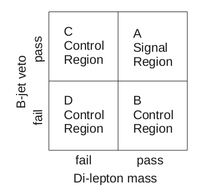
The signal region is defined as that when the cuts relating to the Higgs decay products are made so as to maintain as much statistics as possible. In this signal region, $ \toptop $ remains a dominant background, contributing around 10 $ \% $ to the total background as shown in the second column of Figure 33. As detailed in the section b-jet veto, it was shown that the b-jet veto was particularly efficient at rejecting $ \toptop $, reducing it by over 60 $ \% $ with respect to the previous cut applied. By explicitly requiring a b-tagged jet the control region B $ ^{\toptop} $ enriched with $ \toptop $ may be established, as shown in the third column of Figure 33 (again showing the numbers of expected events after the Higgs decay product selection). It shows that although this control region consists mostly of $ \toptop $, approximately 70 $ \% $, there are other contributions to the total background, particularly from backgrounds with a Z. In order to try and reduce this background, one possibility is to reverse the di-lepton mass cut. To do this a second control region, C $ ^{\toptop} $, is defined by reversing the di-lepton mass cut i.e. $ |\mll-\mZ| > $ 15 $ \Gcs $ but requiring 60 < $ \mll $ < 150 $ \Gcs $. The result of this change in the selection, is shown in the fourth column of Figure 33. In this region significant contamination from W+jets background becomes a problem. However, by requiring both a b-tagged jet and reversing the di-lepton mass window cut, a much purer (over 90 $ \% $ of the total background) $ \toptop $ control region (D $ ^{\toptop} $ ) is defined, as shown in the fifth column of Figure 33. Using the number of $ \toptop $ expected in each control region, the contribution of $ \toptop $ in the signal region is predicted to be 3.94 $ \pm $ 0.19 compared to 3.69 $ \pm $ 0.15 measured, showing agreement within errors and indicating the methodology adopted works. If instead however, the total background values in each control region are used in the estimate of the $ \toptop $ contribution in the signal region, its value is overestimated. This is due to contributions from other backgrounds in the B $ ^{\toptop} $ and C $ ^{\toptop} $ control regions. For the same reason, using the ABCD method with the data leads to an over estimate of the predicted $ \toptop $ contribution in the signal region. However, if region D $ ^{\toptop} $ is considered, a total background of 11.67 $ \pm $ 0.48 events are expected, of which 10.86 $ \pm $ 0.26 are $ \toptop $ and 10 events are observed in the data. This is within the 25 $ \% $ normalisation error assumed for the $ \toptop $ background.

Figure 33: Number of normalised events (33.4 $ \pb $) after the full selection for the $ \mH $ = 200 $ \Gcs $ signal, each background and total background. Included is the observed data events. The number of events are quoted for the nominal selection A $ ^{\toptop} $ and top control regions B,C,D $ ^{\toptop} $.

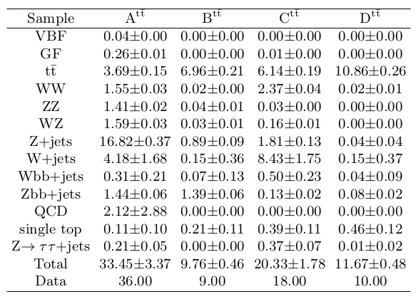
Experimental Uncertainties

In addition to the theoretical uncertainties described previously, it is expected that uncertainties relating to detector performance, mainly caused by misalignment, extra material in the detector and mis-calibration, will be relevant for this analysis as it relies heavily on all the major sub-detectors of the detector. In the following several sources of uncertainty are investigated. The uncertainties used are derived from the relevant performance group or where not available follow [20]. Where possible, official tools provided by the performance groups have been used to assess their effect. In each case the effect of the uncertainty is measured by repeating the analysis for each systematic effect in turn and comparing the overall percentage difference in yield for each background and the total background. The uncertainty on the signal is estimated by repeating the analysis for the $ \mH $ = 200,400,600 $ \Gcs $ signal samples. The final signal uncertainties used come from the $ \mH $ = 200 $ \Gcs $ sample for the low mass selection and the average of the results from the $ \mH $ = 400,600 $ \Gcs $ samples for the high mass selection.

Luminosity

The uncertainty on the luminosity has been measured in [42] and is estimated to be 3.4 $ \% $.

Energy Scale

The energy scale of electrons and muons is expected to affect the selection relating to the Higgs decay products. In particular it has been shown that the di-lepton mass window cut provides lots of discrimination over background, which may be worsened when uncertainty on electron and muon energy scales is taken into account. However, it is expected that this effect will be small because of the high accuracy with which electrons and muons are measured. To estimate the effect of the uncertainty on the electron and muon energy scales, the analysis was repeated and the energy scale of electrons and muons systematically shifted up and down independently. For electrons, as recommended by the e $ \gamma $ performance group [30], a 1(3) $ \% $ uncertainty on the energy scale of electrons in the barrel(end-cap) was assumed. For muons the energy scale uncertainty was assumed to be 1 $ \% $.

In the same way that the energy scale of electrons and muons may affect the acceptance of the analysis with regard to variables related to the Higgs decay products, similarly uncertainty on the jet energy scale is likely to affect the selection related to the VBF remnants. For this reason, the analysis was repeated varying the jet energy scale up and down according to the uncertainty recommendations from the jet $ \etmiss $ performance group. This is implemented using the official Jet Energy Uncertainty Provider [43] [44] which provides a correction to the energy scale of a jet as a function of its $ \pt $ and $ \eta $. Typically, the jet energy uncertainty for jets with $ \pt < $ 100 $ \Gc $ is 8(9) $ \% $ and 6(7) $ \% $ for jets with $ \pt > $ 100 $ \Gc $ in the central(endcap) region [43].

When changing the energy scale of the objects discussed, the effect was propagated to $ \etmiss $ by recalculating the $ \etmiss $ components after modifying the reconstruction performance of the relevant physics object. The effect of changing the electron, muon and jet energy scales is summarised in Figure 34. The effect of changing the jet energy scales has the largest effect. This is largely because the uncertainty on the jet energy scale is greatest. For the same reason the effect of changing the electron energy scale is larger than changing the muon energy scale.

In the signal it is clear that the change in event yield is dominated by the effect of the jet energy scale, in each case the effect of the electron and muon energy scale uncertainties is always less than 1 $ \% $. To this end, for the signal the effect of the electron and muon energy scales is neglected. In addition, because the effect of jet energy scale uncertainty is by far the dominant effect compared to all other detector related uncertainties investigated for the signal, these other effects are neglected. For the low mass selection, increasing the jet energy scale gives rise to an increase in efficiency of around 7 $ \% $, whereas decreasing the jet energy scale sees a decrease in events by around 17 $ \% $. A value of $ \pm $ 12 $ \% $ is assumed. For the high mass selection, the signal appears to be less affected by changes in the jet energy scale. An uncertainty of $ \pm $ 5.5 $ \% $ on the signal rate due to jet energy scale uncertainty in the high mass selection is used.

For the background, the effect of the electron/muon energy scale uncertainty is seen to have a non-negligible effect on total background rate. In the low mass selection, for electrons, a roughly symmetric change in total background yield, of $ \pm $ 9 $ \% $ is observed when increasing/decreasing the electron energy scale. The same trend is true when changing muon energy scale, although the shift down in efficiency is approximately half the effect of the shift up. A value in between these two results is assumed and as such the background uncertainty due to muon energy scale uncertainty is approximated as $ \pm $ 5 $ \% $. Considering the events selected in the analysis either contain two electrons or muons it does not make sense to consider the electron and muon energy scale uncertainties independently. As such, a conservative estimate for the total background uncertainty of $ \pm $ 9 $ \% $ is assumed in the low mass selection, due to the combined electron and muon energy scale uncertainties.

In the high mass selection, the effect of changing the electron and muon energy scales is less pronounced. Following a similar argument to that used for the low mass selection, the combined electron and muon energy scale uncertainty gives an uncertainty on the total background rate in the high mass selection of $ \pm $ 3.5 $ \% $.

The effect of changing jet energy scale appears to have a large effect on the total background rate, giving rise to an increase in total background of over 20 $ \% $ in the low mass selection in the case of decreasing jet energy scale. The effect of increasing background rate with decreasing jet energy scale is caused by the CJV cut accepting more events in this scenario. The largest effect of this kind is seen for the Z+jets background, which increases by over 50 $ \% $. Since this is a major background, this dominates the overall change in background, giving rise to the net increase in total background rate observed. In contrast, when increasing the jet energy scale a much lower change on total background is observed, of a few percent. In this case, despite all other background rates increasing, a net decrease in Z+jets background is observed. This is again caused by the CJV cut, in this case leading to an increased suppression of high jet multiplicity Z events. Again because it is a dominant background, the decrease in Z rate compensates for the increase in background rate from other processes, giving a smaller net change in total background.

Figure 34: Relative changes (%) in efficiency of the optimized selections for $ \mH $ = 200, 400, 600 $ \GeV $ signal samples, each individual background and total background when the energy scale of electrons, muons and jets is varied as detailed. The table includes values for the optimized low and high mass selections. Values are in %.

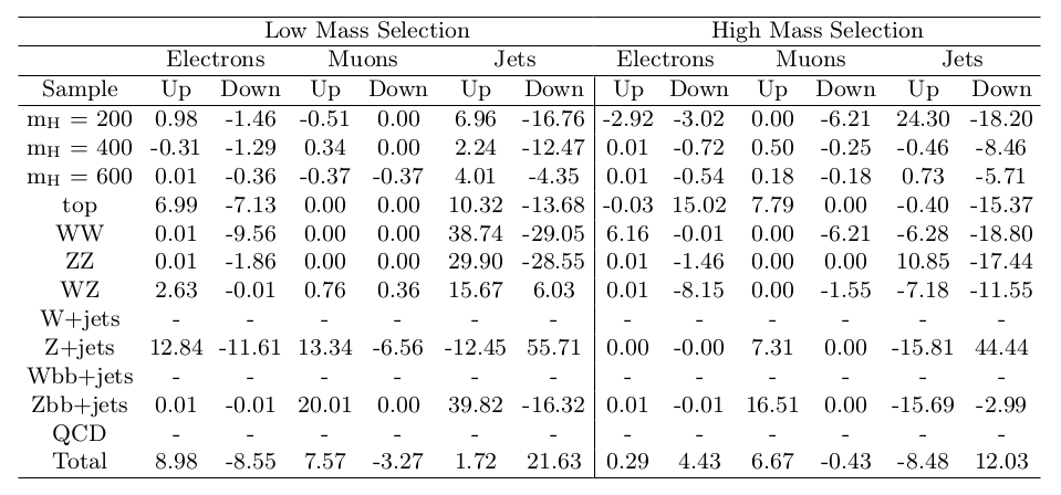
In the high mass selection a similar trend is observed, although the increase in background rate by decreasing jet energy scale is less pronounced, guided by a lower increase in Z+jets background. The effect of increasing jet energy scale leading to a net decrease in background rate is now observed for both $ \toptop $ and Z, driving the observed net decrease in total background of 9 $ \% $. Applying an approximate average to the shifts observed, the uncertainty on the total background rate due to jet energy scale uncertainty, for the low and high mass selections is taken to be $ \pm $ 10 $ \% $.

Energy Resolution

In the following the effect of electron, muon and jet energy resolution uncertainties on the analysis are investigated. In each case, re-calculation of $ \etmiss $ components was made in the same way as was done when looking at the effect of energy scale. In order to estimate the effect of electron energy resolution, the recommendations from the $ e\gamma $ performance group were used [30]. The energy of electrons was corrected by adding $ \Delta E $, found using a randomly distributed Gaussian with width $ \sigma $ $$ \begin{equation} \sigma = \sqrt{(S(1+S_{error})\sqrt{E_{cluster}})^{2} + (C(1+C_{error})E_{cluster})^{2} - (S\sqrt{E_{cluster}})^{2}-(CE_{cluster})^{2} } \label{eqn_ElectronSystResolSigma} \end{equation} $$ where S=0.2 represents the electromagnetic calorimeter sampling term, C=0.007 its constant term and S $ _{error} $ = $ \pm $ 20 $ \% $ and C $ _{error} $ = $ \pm $ 100(400) $ \% $ ( $ |\eta_{cluster}| $ <( $ \geq $ ) 1.37) their respective errors. $ E_{cluster} $ is the cluster energy.

The effect of changing the $ \pt $ resolution of muons was investigated by smearing the $ \pt $ of muons measured in the inner detector and muon spectrometer, applying a +1 $ \sigma $ variation. The effect of varying the jet energy resolution was investigated using the recommendations from the Jet $ \etmiss $ group. This provides a correction to a jet's energy based on its $ \pt $ and $ \eta $.

The effect of the uncertainty on the electron and muon energy resolutions is of similar magnitude in the low mass selection. A value of +5 $ \% $ uncertainty on total background rate is assumed for the combined electron and muon energy resolution uncertainty. In contrast the uncertainty on jet energy resolution leads to a -9 $ \% $ shift in total background. Because the selection used in this study requires electrons/muons and jets and the corresponding uncertainties stated above are one sided and have opposite effects, the overall effect due to the combined energy resolution uncertainty of electrons/muons and jets is a -4 $ \% $ uncertainty on total background rate. The associated systematic uncertainty is therefore taken as $ \pm $ 2 $ \% $. Using a similar approach for the high mass selection an effect of -2 $ \% $ is observed, taking into account the +5 $ \% $ increase and -7 $ \% $ decrease in total background expected from the uncertainty due the electron and muon/jet energy resolution respectively. The associated systematic uncertainty is taken to be $ \pm $ 1 $ \% $.

Reconstruction Efficiency

As discussed, for electrons the Monte Carlo reconstruction efficiency is overestimated compared to that in the data and as such a correction was applied. No correction was applied for muon efficiency. The effect of the uncertainty on the reconstruction and identification efficiency of electrons and muons on the analysis was investigated assuming a uncertainty of 2.3(1) $ \% $ respectively. This was implemented by applying an additional 4.6(2) $ \% $ additional weighting up and down for events satisfying the lepton selection in the $ \ztoee $ ( $ \ztomm $ ) channels respectively. These uncertainties were taken from [20].

Overall the effect on the total background rate is of the order a few percent, for both the low and high mass selections. The combined uncertainty on total background rate due to electron and muon reconstruction efficiency uncertainty is taken to be $ \pm $ 2 $ \% $.

B-tagging Efficiency

The uncertainty on b-tagging efficiency is expected to be important for this analysis as one of the main backgrounds is top, involving decays to b hadrons. Efficient rejection of this background relies on accurate b-tagging algorithms. The uncertainty on the b-tagging efficiency is investigated using the recommendations from the b-tagging performance group [45]. In this method each jet is assigned a ($ \pt $ and $ \eta $ dependent) scale factor. The scale factor takes on a different form depending on whether the jet is tagged by the SV0 algorithm (i.e. has SV0 weight > 5.72 in this analysis) or not. In addition the form of the scale factor is different depending on the Monte Carlo truth nature of the associated jet, i.e. if it is identified as derived from b quarks. In this analysis the procedure of identifying the truth origin of each jet was estimated using the quark flavour of the closest matched truth quark in $ \Delta R $. As expected, increasing the b-tagging efficiency leads to the weight of jets being made larger, indicating an expected decrease in total background because of the b-jet veto cut. The opposite scenario is shown to occur when decreasing the b-tagging efficiency.

Changing the b-tagging efficiency is shown to have negligible effect on all processes considered apart from top and Zbb backgrounds, for which increases of up to 30,10 $ \% $ in their respective yields is expected by decreasing the b-tagging efficiency. The overall change in the total background rate is expected to be more pronounced in the high mass selection by a few percent to approximately 10 $ \% $. This is explained by the contribution of top to the total background in the high mass selection being larger compared to that in the low mass selection. Taking into account the differences when shifting up and down, the uncertainties on the total background rate for the low and high mass selections, due to b-tagging efficiency uncertainty, are taken to be $ \pm $ 7.5 $ \% $ and $ \pm $ 9 $ \% $ respectively.

Total Systematic Uncertainty

The sources of systematic uncertainty investigated and their associated values for the signal and total background, for the low and high mass selections are summarised in Figure 35. The total systematic uncertainty on the signal and total background rate in each selection is obtained by adding the rate uncertainties derived from considering each systematic uncertainty in quadrature. In the low mass selection, the total estimated systematic uncertainty on the signal rate is $ \pm $ 14 $ \% $ and on the total background rate it is $ \pm $ 18 $ \% $. For the high mass selection the estimated systematic uncertainty on the signal rate is $ \pm $ 9 $ \% $ and on the total background rate is $ \pm $ 17 $ \% $. The effect of these uncertainties on the signal significance Z=s/ $ \sqrt{b} $ is shown in Figure 36. The largest impact is observed where the low mass selection is applied, for Higgs masses less than 300 $ \Gcs $. Here approximately a 5 $ \% $ change in signal significance is observed. A negligible impact is observed for masses above 300 $ \Gcs $, owing to more similar uncertainties on signal and background rates for the high mass selection. With improvements in understanding of the detector response and modelling of physics interactions, these uncertainties will be reduced.

Figure 35: Summary of each systematic effect considered on the signal and background for the low and high mass selections. Values are in $ \% $.

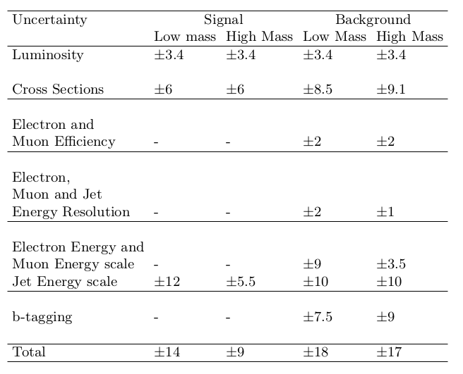
Figure 36: Effect of systematics on signal significance as a function of Higgs mass [GeV].

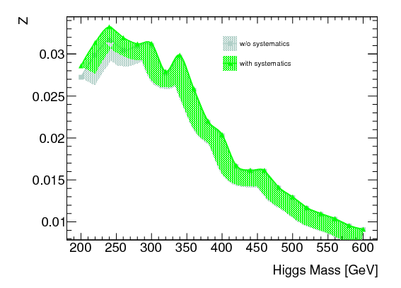
Pile- up

The selection with regard to variables relating to the Higgs decay products has been shown to be largely independent of the pile-up levels seen in the 2010 data, for the selection defined. However, discrepancies were observed when considering the VBF selection and this was attributed to pile-up because of the better observed agreement between data and pile-up reweighted Monte Carlo for the associated variable distributions. Because of insufficient statistics in the pile-up samples available, a detailed study of the effect of pile-up cannot be made with the full selection. In the following an attempt is made to estimate the effect of pile-up on the analysis by comparing the final number of events after applying the (low mass) selection relating to the VBF selection only. This indicates that pile-up at the level considered gives rise to +21 $ \% $ shift in total background rate, largely due to a large net increase in Z+jets background. This highlights the importance that pile-up is likely to have in this channel and that further studies will need to be done to better estimate its effect. With regard to this analysis, it was observed that the main discrepancy between non pile-up and pile-up Monte Carlo was due to the $ \Delta\eta $ distribution. Since this is included in the high mass selection (where no CJV or cut on tag-jets mass is made) the +21 $ \% $ shift in total background rate is assumed for both the low and high mass selections. This is applied not as a systematic but as a shift in the total background rate. No change in the signal rate for the masses tested was observed. The effect on the signal significance Z=s/ $ \sqrt{b} $ is shown in Figure 37. As expected the effect is to reduce signal significance. For Higgs masses lower than 300 $ \Gcs $, where the low mass selection is applied a larger effect is observed because of the slightly higher background level.

Figure 37: Estimated effect of pile-up on signal significance as a function of Higgs mass [GeV].

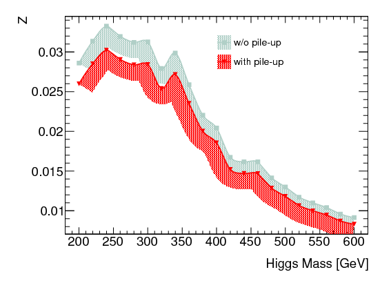
Results in form of Limits

Typically the results of a search are analysed by making a statement about how well the observed results agree or disagree with different hypotheses. In a search for a signal, the null (background only) hypothesis corresponds to the absence of this signal and the alternative corresponds to the signal plus background hypothesis. A test statistic is used to distinguish between the different hypotheses. In the following this is based on the profile likelihood ratio.

The total number of observed events (signal s, background b) is assumed to be distributed according to a Poisson distribution with mean $ \mu $ s+b, where $ \mu = \sigma/\sigma_{SM} $ is the signal strength with $ \mu = $ 0 corresponding to the absence of signal and $ \mu = $ 1 to a signal rate as expected by the SM. Free parameters other than $ \mu $ are referred to as nuisance parameters. Because of the low number of expected signal and background events, in this study the only nuisance parameter ($ \theta $) considered is the expected number of background events. It is also assumed to be distributed according to a Poisson distribution. A likelihood function $ L(\mu,\theta) $ is then defined as the product of these Poisson probabilities and the profile likelihood ratio as $$ \begin{equation} \lambda(\mu) = \frac{L(\mu,\hat{\!\hat{\theta}})}{L(\hat{\mu},\hat{\theta})} \hspace{50pt} (\mu \ge 0) \label{red} \end{equation} $$ where $ \hat{\mu} $ and $ \hat{\theta} $ represent the maximum likelihood estimators of $ \mu $ and $ \theta $. $ \hat{\!\hat{\theta}} $ denotes the conditional maximum likelihood estimator of $ \theta $ when maximizing $ L $ for a specific value of $ \hat{\mu} $. The test statistic is then defined by $$ \begin{equation} q_{\mu} = -2\ln\lambda(\mu) \label{eqn_qmu} \end{equation} $$ The upper limit on the signal cross section is calculated for each tested Higgs mass point using the $ CL_{\mathrm{s}} $ method [46], in which the $ CL_s{} $ value is defined as $$ \begin{equation} CL_{\mathrm{s}} = \frac{CL_{\mathrm{s+b}}}{CL_{\mathrm{b}}} \label{eqn_cls} \end{equation} $$

where $ CL_{s+b} $ (CL $ _{b} $ ) is the probability under the assumption of the signal plus background (background) hypothesis that a value of the corresponding test statistic is found with equal or lesser compatibility with the signal plus background (background) model compared to the value of the test statistic observed. This corresponds to the p-value of the signal plus background (background) hypothesis. The upper limits are set to the 95 $ \% $ C.L. on the signal cross section at each Higgs mass by evaluating the $ CL_{s} $ value for a range of $ \mu $ values and finding the corresponding $ \mu $ such that the $ CL_{s} $ value converges to 0.05. If this $ \mu $ has a value of less than one the signal is regarded as excluded at the 95 $ \% $ C.L.

The 95 $ \% $ C.L. limits on the signal cross section relative to the SM prediction are shown in Figure 38. The integrated luminosity corresponds to 33.4 $ \pb $ of data collected in 2010. The most stringent limits are found in the mass region between 250 and 350 $ \Gcs $. This corresponds to the high mass end of the low mass selection, giving the best compromise between increased signal discrimination and the reduction in signal cross section with increasing Higgs mass. Outside this region, with decreasing Higgs mass the limits are worsened by the poorer signal over background discrimination of the cuts used while for higher masses, the same trend is observed but is largely due to decreasing signal cross section with increasing Higgs mass. Overall the limits are slightly better than 1/10 the expected confidence limits obtained for the gluon fusion analysis [20]. This indicates that the VBF specific analysis considered here is at least as competitive as the GF analysis, when the order of magnitude lower cross section for the VBF signal is taken into account.

Figure 38: Expected and observed VBF signal cross section exclusion limits relative to the predicted SM cross section as a function of Higgs boson mass [GeV] taking into account the optimized selection with the effect of pile-up (systematic uncertainties quoted in the section Total Systematic Uncertainty also taken into account). Integrated luminosity corresponds to 33.4 $ \pb $ of data collected in 2010. The dashed line shows the expected exclusion while the green and yellow bands show the associated $ \pm1\sigma $ and $ \pm2\sigma $ statistical errors. The solid line represents the observed limits.

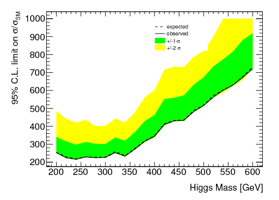
Conclusions

The Higgs boson was until its discovery in 2012 the last remaining missing piece to the SM which had yet to be experimentally verified. The ATLAS experiment is one of two experiments at the LHC which is being used to try and find evidence of its existence and measure it's properties.

This study made a first dedicated look into the sensitivity of the $ \htollnunu $ final state where the Higgs boson is produced by the VBF mechanism, for Higgs boson masses between $ \mH $ = 200-600 $ \Gcs $. The analysis was performed using fully simulated Monte Carlo samples including trigger information. The performance of the reconstruction of electrons, muons and jets in the signal was shown to be robust against the main backgrounds. In order to take into account the changing signal properties with increasing Higgs mass, a low and high mass selection were developed, with the best performing analysis chosen as a function of Higgs mass. In the low mass selection, the lower $ \etmiss $ levels in the signal mean that it relies more heavily on the unique properties of tag-jets associated with the VBF topology to suppress background. In contrast the high levels of $ \etmiss $ in higher Higgs boson mass signals, was shown to give the most powerful discrimination over the background. An optimization procedure was performed on each of the selections and yielded of the order of a 10 $ \% $ improvement in signal significance over the Higgs masses investigated relative to the baseline selections outlined.

The main backgrounds to both selections have been identified as $ \toptop $ and Z+jets, which together make up $ \approx $ 80 $ \% $ of the total background in both the low and high mass selections. Methods were explored to try and estimate their contribution using data driven techniques. The method used to estimate $ \toptop $ verified the uncertainty assumed on the $ \toptop $ cross section. The effect of various systematic uncertainties was taken into account and the combined systematic uncertainty predicted to be of the same order as statistical uncertainty, $ \approx $ 20 $ \% $.

95 $ \% $ C.L. limits on the signal cross section relative to the SM prediction as a function of Higgs boson mass showed that this analysis appears to be most sensitive to Higgs masses between 250 and 350 $ \Gcs $. Taking into account its order of magnitude lower cross section, this analysis was shown to have a similar performance to the GF analysis [20].

At the time of this study, although regions of the SM Higgs mass had been excluded to 95 $ \% $ C.L., regions of un-excluded Higgs mass remained in the mass region considered in this analysis. Although this would have needed to be re-evaluated using more data, the studies in this study showed this channel may have effectively contributed to this search.

Bibliography

P. W. Higgs. Broken Symmetries and the Masses of Gauge Bosons, Phys. Rev. Lett., 13, pp. 508-509, doi: 10.1103/PhysRevLett.13.508, 1964.
F. Englert and R. Brout. Broken Symmetry and the Mass of Gauge Vector Mesons, Phys. Rev. Lett., 13, pp. 321-322, doi: 10.1103/PhysRevLett.13.508, 1964.
G. S. Guralnik, C. R. Hagen and T. W. B. Kibble. Global Conservation Laws and Massless Particles, Phys. Rev. Lett., 13, pp. 585-587, doi: 10.1103/PhysRevLett.13.508, 1964.
K. Nakamura et al.. Review of Particle Physics, Comput. Phys., G37, pp. 075021, doi: 10.1088/0954-3899/37/7A/075021, 2010.
V. B. a. R. Phillips. Collider Physics, in Collider Physics, 1996.
F. Halzen and A. D. Martin. Quarks and Leptons: an Introductory Course in Modern Particle Physics, John Wiley and Sons, 1984.
T. A. Collaboration. Update of the Combination of Higgs Boson Searches in Pp Collisions at $ \sqs $ =7 TeV With the ATLAS Experiment at the LHC, ATL-PHYS-INT-2011-049, 2011.
L. H. C. S. W. Group, S. Dittmaier, C. Mariotti, G. Passarino and T. (Eds.). Handbook of LHC Higgs Cross Sections: 1. Inclusive Observables, CERN-2011-002, CERN, Geneva, 2011.
A. Djouadi. The Anatomy of Electro-Weak Symmetry Breaking. I: the Higgs Boson in the Standard Model, Phys. Rev. Lett., 457, pp. 1-216, doi: 10.1016/j.physrep.2007.10.004, 2008.
J. P. Blewett. 200 GeV Intersecting Storage Accelerators, Proceedings of the 8th International Conference on High-Energy Accelerators, 1971.
T. ATLAS. The ATLAS Experiment at the CERN Large Hadron Collider, Journal of Instrumentation 3, S08003, 2008.
T. ATLAS. ATLAS Detector and Physics Performance: Technical Design Report, 2008 JINST 3 P03001,ATLAS-TDR-014, 1999.
G. Aad et al.. Expected Performance of the ATLAS Experiment - Detector, Trigger and Physics, arXiv, 2009.
T. ATLAS. Inner Detector Technical Design Report Vol I, CERN/LHCC/97-17, 1997.
T. ATLAS. Inner Detector Technical Design Report Vol II, CERN/LHCC/97-17, 1997.
T. ATLAS. Muon Spectrometer Technical Design Report, CERN/LHCC/97-17, 1997.
P. Jenni, M. Nessi, M. Nordberg and K. Smith. ATLAS High-Level Trigger, Data-Acquisition and Controls: Technical Design Report, Technical Design Report ATLAS, CERN, 2003.
A. Gesualdi-Mello et al.. Overview of the High-Level Trigger Electron and Photon Selection for the ATLAS Experiment at the LHC, IEEE Trans. Nucl. Sci., 2002.
S. Angelidakis et al.. Search for a Standard Model Higgs in the Mass Range 200-600 GeV in the Channels $ \htollnunu $ and $ \htollqq $, ATL-PHYS-INT-2011-049, 2011.
T. ATLAS. Search for a Standard Model Higgs Boson in the Mass Range 200-600 GeV in the Channels $ \htollnunu $ and $ \htollqq $ With the ATLAS Detector, ATL-PHYS-INT-2011-049, 2011.
Gabrielli, E. a. Mele and Barbara. Testing Effective Yukawa Couplings in Higgs Searches at the Tevatron and LHC, Phys.Rev., 20010.
M. A. Dobbs et al.. Les Houches Guidebook to Monte Carlo Generators for Hadron Collider Physics, arXiv, 2004.
S. Frixione and B. R. Webber. Matching NLO QCD Computations and Parton Shower Simulations, JHEP, 06, pp. 029, 2002.
T. Sjostrand, S. Mrenna and P. Z. Skands. PYTHIA 6.4 Physics and Manual, JHEP, 05, pp. 026, doi: 10.1088/1126-6708/2006/05/026, 2006.
P. Golonka and Z. Was. PHOTOS Monte Carlo: a Precision Tool for QED Corrections in Z and W Decays, Eur Phys J C, C45, pp. 97-107, doi: 10.1140/epjc/s2005-02396-4, 2006.
Z. Was. TAUOLA the Library for Tau Lepton Decay, and KKMC/KORALB/KORALZ/... Status Report, Nucl. Phys. Proc. Suppl., 98, pp. 96-102, doi: 10.1016/S0920-5632(01)01200-2, 2001.
M. L. Mangano, M. Moretti, F. Piccinini, R. Pittau and A. D. Polosa. ALPGEN, a Generator for Hard Multiparton Processes in Hadronic Collisions, JHEP, 07, pp. 001, 2003.
G. Corcella et al.. HERWIG 6.5: an Event Generator for Hadron Emission Reactions With Interfering Gluons (including Supersymmetric Processes), JHEP, 01, pp. 010, 2001.
M. Aharrouche et al.. Expected Electron Performance in the ATLAS Experiment, CERN, ATL-PHYS-INT-2010-126, 2010.
ATLAS. ATLAS Egamma Combined Performance Group, Energy Scale and Resolution Recommendations, CERN, 2010.
ATLAS. ATLAS Egamma Combined Performance Group, Efficiency Measurements, CERN, 2010.
ATLAS. ATLAS Muon Combined Performance Group, Guidelines for Analysis in Release 15, CERN, 2010.
F. Cerutti, C. Gatti, P. Kluit, O. Kortner, W. Liebig, J. Liu, G. Salamanna, A. Salvucci, E. v. d. Poel and J. Zhu. Muon Momentum Resolution in First Pass Reconstruction of Pp Collision Data Recorded by ATLAS in 2010, CERN, ATLAS-COM-CONF-2011-003, 2011.
T. ATLAS. Determination of the Muon Reconstruction Efficiency in ATLAS at the Z Resonance in Proton-Proton Collisons at $ \sqs $ =7 TeV, CERN, ATLAS-CONF-2011-008, 2011.
B. Heinemann, F. Hirsch and S. Strandberg. Performance of the ATLAS Secondary Vertex B-Tagging Algorithm in 7 TeV Collision Data, CERN, ATLAS-COM-CONF-2010-042, 2010.
T. ATLAS. Measurement of the Top Quark-Pair Production Cross Section With ATLAS in Pp Collisions at $ \sqs $ =7 TeV, Eur Phys J C, C71, pp. 1577, doi: 10.1140/epjc/s10052-011-1577-6, 2011.
ATLAS. Jet, Etmiss bad jets reccomendations, CERN, 2010.
T. A. Collaboration. Measurement of Missing Tranverse Energy, CERN, ATL-PHYS-PUB-2009-016. ATL-COM-PHYS-2009-118, 2009, Draft PUB Note for 'Measurement of Missing Transverse Energy in ATLAS' Chapter (J13).
T. ATLAS. Performance of the Missing Transverse Energy Reconstruction and Calibration in Proton-Proton Collisions at a Center-of-Mass Energy of 7 TeV With the ATLAS Detector, CERN, ATLAS-CONF-2010-057, 2010.
K. Cranmer, Y. Fang, B. Mellado, S. Paganis, W. Quayle et al.. Prospects for Higgs Searches Via VBF at the LHC With the ATLAS Detector, arXiv, 2004.
Cowan, G. a. Cranmer, K. a. Gross, E. a. Vitells and Ofer. Asymptotic formulae for likelihood-based tests of new physics, The European Physical Journal C, 2011.
T. A. Collaboration. Updated Luminosity Determination in pp Collisions at $ \sqs $ =7 TeV Using the ATLAS Detector, CERN, 2011.
T. ATLAS. Jet Energy Scale and Its Systematic Uncertainty for Jets Produced in Proton-Proton Collisions at $ \sqs $ =7 TeV and Measured With the ATLAS Detector, CERN, ATLAS-CONF-2010-056, 2010.
T. ATLAS. Update on the Jet Energy Scale Systematic Uncertainty for Jets Produced in Proton-Proton Collisions at $ \sqs $ =7 TeV Measured With the ATLAS Detector, CERN, ATLAS-CONF-2011-007, 2011.
M. Bosman, L. Fiorini, C. Helsens, A. Juste, L. Mir, J. Nadal and V. Vorwerk. Weighting Method to Propagate Heavy-Flavor Tagging Calibrations and Related Uncertainties, CERN, ATL-COM-PHYS-2010-331, 2010.
A. L. Read. Presentation of Search Results: the CL(s) Technique, Comput. Phys., G28, pp. 2693-2704, doi: 10.1088/0954-3899/28/10/313, 2002.