Aim of analysis

This work is based on that performed by Chris Bow [1] which was implemented using R. The aim of this project is to convert the analysis to Python and investigate the dataset further.

Facebook Advertising Platform

Facebook users provide Facebook with a huge wealth of information which can be used to build up a detailed profile of users personal information, habits and interests. Advertisers using Facebook as a platform for their adverts can then tailor their advertising strategy appropriately, perhaps focussing on particular groups of users with similar attributes for a particular product or concentrating on presenting different features of their product to the appropriate groups.

Optimizing the advertising strategy may well mean different things for different businesses, but in each case the end goal of any analysis is to provide actionable answers to the relevant questions which can drive business performance, however that may be measured. Common aims may be to:

• improve brand awareness
• improve future purchases based on adding customer lifetime value
• maximise the amount of revenue returned for the minimum expenditure.

Description of Data

The data was provided in csv format and available from Kaggle [1]. The data consists of the following variables:

• ad_id, unique ID for each ad.
• xyz_campaign_id, an ID associated with each ad campaign of XYZ company.
• fb_campaign_id, an ID associated with how Facebook tracks each campaign.
• age, age of the person to whom the ad is shown.
• gender, gender of the person to whom the add is shown
• interest, a code specifying the category to which the persons interest belongs.
• Impressions, the number of times the ad was shown.
• Clicks, number of clicks on for that ad.
• Spent, Amount paid by company xyz to Facebook, to show that ad.
• Total conversion, Total number of people who enquired about the product after seeing the ad.
• Approved conversion, Total number of people who bought the product after seeing the ad.

Creating features relevant for ad analysis

The following variables are common metrics used in ad analysis and will be added to the dataset:

• Click-through-rate (CTR), which is the percentage of how many impressions became clicks. A high CTR (2 percent as benchmark) is indicative of adverts being well recieved by a relevant audience. A low CTR suggests either both or one of these factors has not been achieved.
• Conversion Rate (CR), is the percentage of clicks that result in a conversion, as defined by the campaign objectives (i.e. sale, contact form completed, downloading an e-book or spending more than a certain time viewing the website).
• Cost Per Click (CPC), on average. This must be considered in combination with other variables (i.e. CR).
• Cost Per Conversion, which combines the CPC and CR metrics.
• Conversion Value, which is how much each conversion is worth. The target conversion value will depend on what the definition of the conversion is and how this is related to revenue returned for example, when maximising revenue is the business aim.
• Return on Advertising Spend (ROAS), which is the revenue returned as a percentage of the advertising spend.
• Cost Per Mille (CPM), which is the cost of one thousand impressions (useful metric when considering brand awareness as business performance metric).

df['CTR'] = (df['Clicks']/df['Impressions']*100)
df['CPC'] = df['Spent']/df['Clicks']

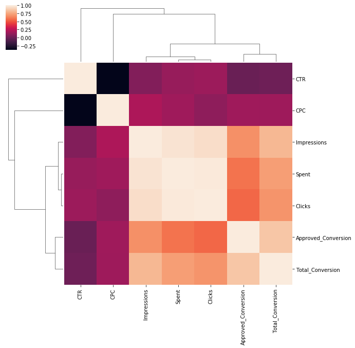
To get an initial idea of how the variables are related, look at the correlation between the following. The result is shown in Figure 1.

subset_df = df[['CTR', 'CPC', 'Approved_Conversion', 'Total_Conversion', 'Impressions', 'Spent', 'Clicks']].copy()

p1 = sns.clustermap(subset_df.corr())
p1.savefig('./figures/plot1.png')

To look at the correlation numerically can also do the following.

corr = subset_df.corr(method='pearson')#.style.format("{:.2}").background_gradient(cmap=plt.get_cmap('coolwarm'), axis=1)
corr
CreateTableHTML('./figures/',corr,'table2')

# plot correlated values
plt.rcParams['figure.figsize'] = [16, 6]

fig, ax = plt.subplots(nrows=1, ncols=2)

ax=ax.flatten()

cols = ['Clicks','Total_Conversion']
colors=['#415952', '#243AB5']#, '#243AB5','#243AB5']
j=0

for i in ax:
    if j==0:
        i.set_ylabel('Spent')
    i.scatter(subset_df[cols[j]], subset_df['Spent'],  alpha=0.5, color=colors[j])
    i.set_xlabel(cols[j])
    i.set_title('Pearson: %s'%subset_df.corr().loc[cols[j]]['Spent'].round(2)+' Spearman: %s'%subset_df.corr(method='spearman').loc[cols[j]]['Spent'].round(2))
    j+=1

plt.savefig('./figures/plot2.png')
plt.show()

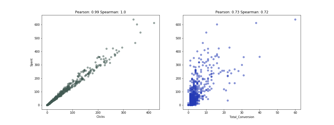
It is reassuring that the higher the spend, the more clicks and although less reliably, the more conversions. However, in order to be able to provide an improvement in the desired business performance, in this case maximising revenue, actionable insights have to be obtained. The data is broken down into different campaigns, which will need to be analysed in turn.

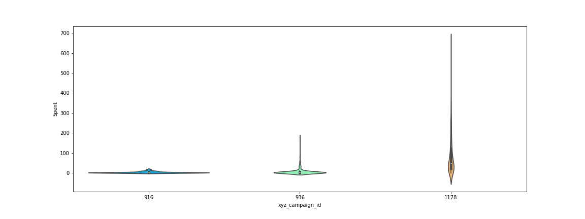
Figure 3 shows campaign 1178 has the biggest spend, so this is the one that will be focussed on further.

Looking at specific campaigns

Campaign 1178

The data for campaign 1178 is shown below

Missing data

The amount of missing data was checked, as shown in the table below which shows the percentage of missing data for each variable. Missing values are only present for the CPC variable, where clicks and spent equal 0, returning NAN.

columns = cam_df.columns
percentage_missing = cam_df.isnull().sum() * 100 / len(cam_df)
table_percentage_missing = pd.DataFrame({'column_name': columns,
                                 'percentage_missing': percentage_missing})

table_percentage_missing

CreateTableHTML('./figures/',table_percentage_missing,'table4')

Distributions among different demographics

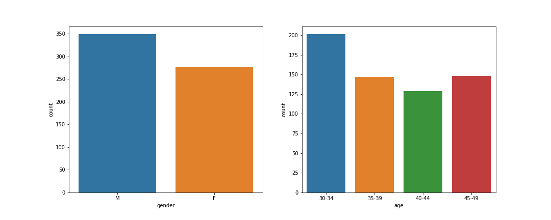
Figure 4 shows basic count distributions for gender and age subgroups. There is no overwhelming unbalanced contributions to these subgroups.

Further feature engineering

When the business aim is to maximise revenue for advertising expenditure, the ROAS metric is very useful. However, this requires the monetary amounts from conversions (Total_conversion) and sales (Approved_conversion) be known. In the following it is a assumed the former is worth £5 and the later £100. Using this the other metrics were calculated and the resulting dataframe head shown below.

cam_df['totConv'] = cam_df.loc[:,'Total_Conversion'] + cam_df.loc[:,'Approved_Conversion']
cam_df['conVal'] = cam_df['Total_Conversion']*5
cam_df['appConVal'] = cam_df['Approved_Conversion'] * 100
cam_df['totConvVal'] = cam_df['conVal'] + cam_df['appConVal']
cam_df['costPerCon'] = round(cam_df['Spent'] / cam_df['totConv'], 2)
cam_df['ROAS'] = round(cam_df['totConvVal'] / cam_df['Spent'], 2)
cam_df['CPM'] = round((cam_df['Spent'] / cam_df['Impressions']) * 1000, 2)
df5 = cam_df.head()

CreateTableHTML('./figures/',df5,'table5')

ROAS of infinity occurs when there are 0 clicks but a conversion. This may have happened because the click wasn't tracked or it occurred at a different time and has been attributed elsewhere. Convert these values to NAN and check for missing data.

Check that this data change now shows up in missing data count.

Analysis by age, gender and interest

In order to improve a similar campaign with a view to maximising revenue return, the variables available in the dataset (in this case age, gender and interest) can be investigated further with respect to the ROAS metric.

Analysis by gender

Box plots of ROAS for Females and Males is shown in Figure 5.

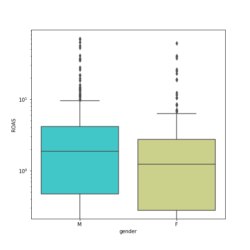
In time, the ROAS is more likely to tend towards the mean, hence this is used subsequently.

• Females mean ROAS 2.81
• Males mean ROAS 4.50

Analysis by interest

grouped_interest = cam_df.groupby('interest').agg({'ROAS':['median','mean'],'Clicks':'sum'}) 
grouped_interest.columns = ['_'.join(x) for x in grouped_interest.columns.ravel()]
grouped_interest = grouped_interest.sort_values(by='ROAS_mean', ascending=0)
grouped_interest.head(10)

CreateTableHTML('./figures/',grouped_interest,'table7')

Although ROAS mean is the metric being used, it is important to take into account the statistical significance of that value. This can be done very approximately by considering the sum of clicks, with a higher sum of clicks for a given interest group making it more likely the calculated ROAS metric is reliable, given the higher population. Given this, interest groups 101, 15 and 21 are considered further.

newdf_grouped_interest = cam_df[(cam_df['interest'] == 101) | (cam_df['interest'] == 15) | (cam_df['interest'] == 21)]
newdf_grouped_interest.head()

Data from these interest groups is further grouped by gender and age group in Figure 6.

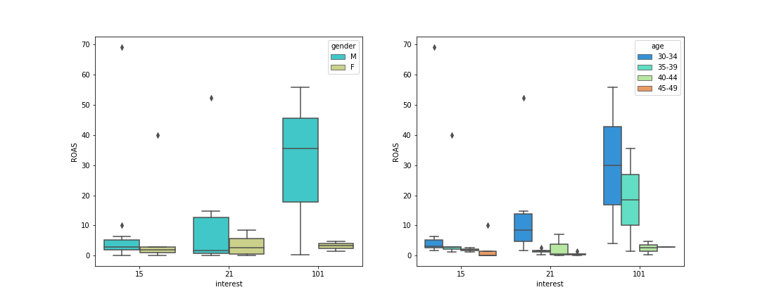
These plots indicate that focussing on males with interest group 101 in the age group 30-34 would be most beneficial to maximising ROAS. However, these plots don't take into account number of clicks for each subgroup, so this is investigated in the following.

#grouped_gender = cam_df.groupby(['interest','gender']).agg({'ROAS':['median','mean'],'Clicks':'sum'}) 
grouped_interest_gender = newdf_grouped_interest.groupby(['interest','gender']).agg({'ROAS':['median','mean'],'Clicks':'sum'}) 
# Using ravel, and a string join, we can create better names for the columns:
grouped_interest_gender.columns = ['_'.join(x) for x in grouped_interest_gender.columns.ravel()]

grouped_interest_gender = grouped_interest_gender.sort_values(by='ROAS_mean', ascending=False)
grouped_interest_gender

CreateTableHTML('./figures/',grouped_interest_gender,'table8')

When considering interest and gender, the table above suggests it might be beneficial to focus more on males with interest in group 101. However, the small number of clicks indicate this high ROAS result could be chance. Overall, when each of the interest groups 101, 21 and 15 are considered, more return is generated from males.

#grouped_gender = cam_df.groupby(['interest','gender']).agg({'ROAS':['median','mean'],'Clicks':'sum'}) 
grouped_interest_age = newdf_grouped_interest.groupby(['interest','age']).agg({'ROAS':['median','mean'],'Clicks':'sum'}) 
# Using ravel, and a string join, we can create better names for the columns:
grouped_interest_age.columns = ['_'.join(x) for x in grouped_interest_age.columns.ravel()]

grouped_interest_age = grouped_interest_age.sort_values(by='ROAS_mean', ascending=False)
grouped_interest_age

CreateTableHTML('./figures/',grouped_interest_age,'table9')

When considering interest and age, the table above suggests it might be beneficial to focus more on people in the 30-34 age group with interest in group 101. However, again, the small number of clicks indicate this high ROAS result could be chance. The group with interest group 15 and age group 30-34 still has a high ROAS but also has much more substantial clicks sum.

Analysis by age

The data is grouped by age and the median, mean and sum of clicks calculated for each group, with the resulting dataframe sorted by ROAS mean descendingly.

grouped_age = cam_df.groupby('age').agg({'ROAS':['median','mean'],'Clicks':'sum'}) 
# Using ravel, and a string join, we can create better names for the columns:
grouped_age.columns = ['_'.join(x) for x in grouped_age.columns.ravel()]

grouped_age = grouped_age.sort_values(by='ROAS_mean', ascending=0)
grouped_age.head(10)

#CreateTableHTML('./figures/',grouped_age,'table10')

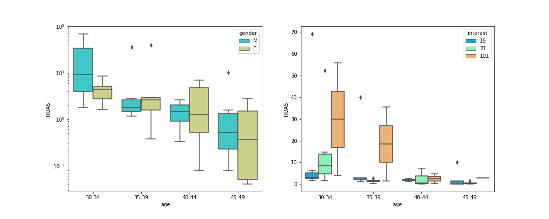
The table above again suggests focussing on the 30-34 age group. Figure 7 shows the ROAS as a function of age group subdivided by gender and interest group (15,21 or 101). Again the 30-34 age group is highlighted, particularly for males and for the interest group 101.

grouped_age_gender = cam_df.groupby(['age','gender']).agg({'ROAS':['median','mean'],'Clicks':'sum'}) 
grouped_age_gender.columns = ['_'.join(x) for x in grouped_age_gender.columns.ravel()]
grouped_age_gender = grouped_age_gender.sort_values(by='ROAS_mean', ascending=False)
grouped_age_gender
CreateTableHTML('./figures/',grouped_age_gender,'table11')

Grouping by gender in addition verifies that the group age group 30-34 is most important to focus on. The least effective age group to focus on would be the 45-49 age group. The gender split in performance accross age groups is less apparent than which was observed for interests.

Analysis by age, gender and interest

The data is grouped by age, interest and gender and the median, mean and sum of clicks calculated for each group, with the resulting dataframe sorted by ROAS mean descendingly. This also indicates that the 30-34 age group is of importance and should be targeted further. However, now because the data has been subdivided so much, statistics available for each subgroup is more limited, making any conclusions less reliable.

Conclusions

This project has been an exploratory data analysis using facebook ad data. It has assumed business performance is determined by absolute return and as such the ROAS metric has been used to try and identify how to generate better performance had a similar campaign been run. Sum of clicks for each group identified was also used as an approximate indicator of the validity of the mean ROAS measured. The findings indicate a similar campaign should:

• focus on the 30-34 age group.
• focus on males.
• focus on groups with interests 15,21 and 101.

• the 45-49 age group.
• females in this age group.

Bibliography

1. C. Bow. An introduction to Facebook ad analysis using R, Kaggle, 2018.